Important: I strongly recommend reading this documentation on the pkgdown documentation website rather than on GitHub! The website includes proper formatting, a dynamic table of contents, an embedded interactive GUI for the tools, full documentation and examples for all functions, and a much better reading experience. Bear in mind that GitHub always displays the latest version of the README (usually a dev version) while the main website is for the latest release version – however, the latest dev section of the website always matches the latest dev GitHub.
1 Introduction
1.1 General introduction
ggDNAvis is an R package that uses ggplot2 to visualise genetic data of three main types:
a single DNA/RNA sequence split across multiple lines,
multiple DNA/RNA sequences, each occupying a whole line, or
base modifications such as DNA methylation called by modified-bases models in Dorado or Guppy.
This is accomplished through main functions visualise_single_sequence(), visualise_many_sequences(), and visualise_methylation() respectively. Each of these has helper sequences for streamlined data processing, as detailed later in the section for each visualisation type.
Additionally, ggDNAvis contains a built-in example dataset (example_many_sequences) and a set of colour palettes for DNA visualisation (sequence_colour_palettes).
As of v1.0.0, aliases are now fully configured so either American or British spellings should work. “Colour” and “visualise” remain the spellings used throughout the code and documentation but “color”, “col”, and “visualize” should also work in all function and argument names (e.g. visualize_single_sequence()). If any American spellings don’t work then please submit a bug report at https://github.com/ejade42/ggDNAvis/issues.
1.2 Installation
The latest release of ggDNAvis is available from CRAN or via github releases. Alternatively, the latest in-development version can be installed directly from the github repository, but may have unexpected bugs.
## Latest release version
install.packages("ggDNAvis")

## Current development build (may have unexpected bugs!)
devtools::install_github("ejade42/ggDNAvis")

## Specific version from github
devtools::install_github("ejade42/ggDNAvis", ref = "v1.0.1")
Throughout this manual, only ggDNAvis, dplyr, and ggplot2 are loaded. The following chunk provides setup for rendering this README page and should NOT be copied verbatim. If you are trying to work through the examples, use the alternative setup chunk below.
## THIS SETUP CHUNK IS FOR THE WEBPAGE AND WILL NOT WORK FOR RUNNING THE EXAMPLES LOCALLY

## Load this package
library(ggDNAvis)

## Load useful tidyverse packages
## These are ggDNAvis dependencies, so will always be installed when installing ggDNAvis
library(dplyr)
library(ggplot2)

## Function for viewing tables throughout this document
## This is not a package data-processing function, it just helps make this document
print_table <- function(data) {
    quoted <- as.data.frame(
        lapply(data, function(x) {paste0("`", x, "`")}),
        check.names = FALSE
    )
    kable_output <- knitr::kable(quoted)
    return(kable_output)
}

## Function for viewing figures throughout this document
view_image <- function(filename) {
    knitr::include_graphics(filename)
}

## Set up file locations
output_location <- "README_files/output/"
display_location <- "https://raw.githubusercontent.com/ejade42/ggDNAvis/v1.0.1/README_files/output/"
knitr::opts_chunk$set(fig.path = output_location)

## Print current ggDNAvis version
cat("Loaded ggDNAvis version is:", as.character(packageVersion("ggDNAvis")))If you are working through the examples, use this setup chunk instead:
## THIS SETUP CHUNK WILL ALLOW YOU TO RUN THE EXAMPLES YOURSELF

## Load pacakges
library(ggDNAvis)
library(dplyr)
library(ggplot2)
library(magick) ## additional - needed for viewing images

## Function for printing tables to console
print_table <- function(data) {
    quoted <- as.data.frame(
        lapply(data, function(x) {paste0("`", x, "`")}),
        check.names = FALSE
    )
    table_output <- tibble(quoted)
    return(table_output)
}

## Function for viewing figures in plot window
view_image <- function(filename) {
    plot(image_read(filename))
}

## File location to output to
output_location <- "PUT YOUR FOLDER NAME HERE ENDING IN A SLASH/"
display_location <- output_location # you probably want these to be the same

## Print current ggDNAvis version
cat("Loaded ggDNAvis version is:", as.character(packageVersion("ggDNAvis")))
1.3 Interactive suite
An interactive GUI-based version of ggDNAvis that runs in a browser is available from the “interactive app” tab of the top navbar of this website, or directly from https://ejade42-ggdnavis.share.connect.posit.cloud/.
This is implemented via a Shiny app, which can also be launched from R on any local computer that has ggDNAvis installed, via the ggDNAvis_shinyapp() function:
The files for the app are stored in the inst/shinyapp/ directory, accessible via system.file("shinyapp/", package = "ggDNAvis").
2 Summary/quickstart
This section contains one example for each type of visualisation. See the relevant full sections for more details and customisation options.
2.1 Single sequence
## Create input sequence. This can be any DNA/RNA string
sequence <- "GGCGGCGGCGGCGGCGGCGGCGGCGGCGGCGGCGGCGGCGGCGGCGGCGGCGGCGGCGGCGGCGGCGGCGGCGGCGGCGGCGGCGGCGGCGGCGGCGGCGGCGGCGGCGGCGGCGGCGGCGGCGGCGGCGGCGGCGGCGGCGGCGGCGGCGGCGGCGGCGGCGGCGGCGGCGGCGGCGGCGGCGGCGGCGGCGGCGGCGGCGGCGGCGGCGGCGGCGGAGGAGGCGGCGGAGGAGGCGGCGGAGGAGGCGGCGGAGGAGGCGGCGGAGGAGGCGGCGGAGGAGGCGGCGGAGGAGGCGGCGGAGGAGGCGGCGGAGGAGGCGGCGGAGGAGGCGGCGGAGGAGGCGGCGGAGGAGGCGGCGGAGGAGGCGGCGGAGGAGGCGGCGGAGGAGGCGGC"

## Create visualisation
## This lists out all arguments
## Usually it's fine to leave most of these as defaults
visualise_single_sequence(
    sequence = sequence,
    sequence_colours = sequence_colour_palettes$bright_pale,
    background_colour = "white",
    line_wrapping = 60,
    spacing = 1,
    margin = 0.5,
    sequence_text_colour = "black",
    sequence_text_size = 16,
    index_annotation_colour = "darkred",
    index_annotation_size = 12.5,
    index_annotation_interval = 15,
    index_annotations_above = TRUE,
    index_annotation_vertical_position = 1/3,
    index_annotation_always_first_base = TRUE,
    index_annotation_always_last_base = TRUE,
    outline_colour = "black",
    outline_linewidth = 3,
    outline_join = "mitre",
    return = FALSE,
    filename = paste0(output_location, "summary_single_sequence.png"),
    force_raster = FALSE,
    render_device = ragg::agg_png,
    pixels_per_base = 100,
    monitor_performance = FALSE
)

## View image
view_image(paste0(display_location, "summary_single_sequence.png"))
2.2 Many sequences
## Read and merge data
fastq_data <- read_fastq(system.file("extdata/example_many_sequences_raw.fastq", package = "ggDNAvis"), calculate_length = TRUE)
metadata   <- read.csv(system.file("extdata/example_many_sequences_metadata.csv", package = "ggDNAvis"))
merged_fastq_data <- merge_fastq_with_metadata(fastq_data, metadata)

## Extract character vector
## These arguments should all be considered, as they are highly specific to your data
sequences_for_visualisation <- extract_and_sort_sequences(
    sequence_dataframe = merged_fastq_data,
    sequence_variable = "forward_sequence",
    grouping_levels = c("family" = 8, "individual" = 2),
    sort_by = "sequence_length",
    desc_sort = TRUE
)

## Create visualisation
## Usually it's fine to leave most of these as defaults
visualise_many_sequences(
    sequences_vector = sequences_for_visualisation,
    sequence_colours = sequence_colour_palettes$bright_deep,
    background_colour = "white",
    margin = 0.5,
    sequence_text_colour = "white",
    sequence_text_size = 16,
    index_annotation_lines = c(1, 23, 37),
    index_annotation_colour = "darkred",
    index_annotation_size = 12.5,
    index_annotation_interval = 3,
    index_annotations_above = TRUE,
    index_annotation_vertical_position = 1/3,
    index_annotation_full_line = FALSE,
    index_annotation_always_first_base = FALSE,
    index_annotation_always_last_base = FALSE,
    outline_colour = "black",
    outline_linewidth = 3,
    outline_join = "mitre",
    return = FALSE,
    filename = paste0(output_location, "summary_many_sequences.png"),
    force_raster = FALSE,
    render_device = ragg::agg_png,
    pixels_per_base = 100,
    monitor_performance = FALSE
)

## View image
view_image(paste0(display_location, "summary_many_sequences.png"))
2.3 Methylation/modification
## Read and merge data
modification_data <- read_modified_fastq(system.file("extdata/example_many_sequences_raw_modified.fastq", package = "ggDNAvis"))
metadata          <- read.csv(system.file("extdata/example_many_sequences_metadata.csv", package = "ggDNAvis"))
merged_modification_data <- merge_methylation_with_metadata(
    modification_data,
    metadata,
    reversed_location_offset = 1
)

## Extract list of character vectors
## These arguments should all be considered, as they are highly specific to your data
methylation_for_visualisation <- extract_and_sort_methylation(
    modification_data = merged_modification_data,
    locations_colname = "forward_C+m?_locations",
    probabilities_colname = "forward_C+m?_probabilities",
    lengths_colname = "sequence_length",
    grouping_levels = c("family" = 8, "individual" = 2),
    sort_by = "sequence_length",
    desc_sort = TRUE
)

## Create visualisation
## Usually it's fine to leave most of these as defaults
visualise_methylation(
    modification_locations     = methylation_for_visualisation$locations,
    modification_probabilities = methylation_for_visualisation$probabilities,
    sequences                  = methylation_for_visualisation$sequences,
    low_colour = "blue",
    high_colour = "red",
    low_clamp = 0.1*255,
    high_clamp = 0.9*255,
    background_colour = "white",
    other_bases_colour = "grey",
    sequence_text_type = "none",
    index_annotation_lines = 1:51,
    index_annotation_colour = "darkred",
    index_annotation_size = 12.5,
    index_annotation_interval = 9,
    index_annotations_above = TRUE,
    index_annotation_vertical_position = 1/3,
    index_annotation_full_line = FALSE,
    index_annotation_always_first_base = TRUE,
    index_annotation_always_last_base = TRUE,
    outline_colour = "black",
    outline_linewidth = 3,
    outline_join = "mitre",
    margin = 0.5,
    return = FALSE,
    filename = paste0(output_location, "summary_methylation_none.png"),
    force_raster = FALSE,
    render_device = ragg::agg_png,
    pixels_per_base = 100,
    monitor_performance = FALSE
)

## View image
view_image(paste0(display_location, "summary_methylation_none.png"))
2.3.1 Methylation showing sequence
## Create visualisation showing sequence
visualise_methylation(
    modification_locations     = methylation_for_visualisation$locations,
    modification_probabilities = methylation_for_visualisation$probabilities,
    sequences                  = methylation_for_visualisation$sequences,
    low_colour = "blue",
    high_colour = "red",
    low_clamp = 0.1*255,
    high_clamp = 0.9*255,
    background_colour = "white",
    other_bases_colour = "grey",
    sequence_text_type = "sequence",
    sequence_text_colour = "black",
    sequence_text_size = 16,
    index_annotation_lines = c(1, 23, 37),
    index_annotation_colour = "darkred",
    index_annotation_size = 12.5,
    index_annotation_interval = 15,
    index_annotations_above = TRUE,
    index_annotation_vertical_position = 1/3,
    index_annotation_full_line = TRUE,
    index_annotation_always_first_base = TRUE,
    index_annotation_always_last_base = FALSE,
    outline_colour = "black",
    outline_join = "mitre",
    modified_bases_outline_linewidth = 3,
    other_bases_outline_linewidth = 1,
    margin = 0.5,
    return = FALSE,
    filename = paste0(output_location, "summary_methylation_sequence.png"),
    render_device = ragg::agg_png,
    pixels_per_base = 100
)

## View image
view_image(paste0(display_location, "summary_methylation_sequence.png"))
2.3.2 Methylation showing probabilities
## Create visualisation showing probabilities
visualise_methylation(
    modification_locations     = methylation_for_visualisation$locations,
    modification_probabilities = methylation_for_visualisation$probabilities,
    sequences                  = methylation_for_visualisation$sequences,
    low_colour = "blue",
    high_colour = "red",
    low_clamp = 0.1*255,
    high_clamp = 0.9*255,
    background_colour = "white",
    other_bases_colour = "grey",
    sequence_text_type = "probability",
    sequence_text_scaling = c(-0.5, 256),
    sequence_text_rounding = 2,
    sequence_text_colour = "white",
    sequence_text_size = 10,
    index_annotation_lines = c(1, 23, 37),
    index_annotation_colour = "darkred",
    index_annotation_size = 12.5,
    index_annotation_interval = 15,
    index_annotations_above = TRUE,
    index_annotation_vertical_position = 1/3,
    index_annotation_full_line = TRUE,
    index_annotation_always_first_base = TRUE,
    index_annotation_always_last_base = FALSE,
    outline_colour = "black",
    outline_join = "mitre",
    modified_bases_outline_linewidth = 3,
    other_bases_outline_linewidth = 1,
    margin = 0.5,
    return = FALSE,
    filename = paste0(output_location, "summary_methylation_probabilities.png"),
    render_device = ragg::agg_png,
    pixels_per_base = 100
)

## View image
view_image(paste0(display_location, "summary_methylation_probabilities.png"))
2.3.3 Methylation showing probability integers
## Create visualisation showing probability integers
visualise_methylation(
    modification_locations     = methylation_for_visualisation$locations,
    modification_probabilities = methylation_for_visualisation$probabilities,
    sequences                  = methylation_for_visualisation$sequences,
    low_colour = "blue",
    high_colour = "red",
    low_clamp = 0.1*255,
    high_clamp = 0.9*255,
    background_colour = "white",
    other_bases_colour = "grey",
    sequence_text_type = "probability",
    sequence_text_scaling = c(0, 1),
    sequence_text_rounding = 0,
    sequence_text_colour = "white",
    sequence_text_size = 10,
    index_annotation_lines = c(1, 23, 37),
    index_annotation_colour = "darkred",
    index_annotation_size = 12.5,
    index_annotation_interval = 15,
    index_annotations_above = TRUE,
    index_annotation_vertical_position = 1/3,
    index_annotation_full_line = TRUE,
    index_annotation_always_first_base = TRUE,
    index_annotation_always_last_base = TRUE,
    outline_colour = "black",
    outline_join = "mitre",
    modified_bases_outline_linewidth = 3,
    other_bases_outline_linewidth = 1,
    margin = 0.5,
    return = FALSE,
    filename = paste0(output_location, "summary_methylation_probability_integers.png"),
    render_device = ragg::agg_png,
    pixels_per_base = 100
)

## View image
view_image(paste0(display_location, "summary_methylation_probability_integers.png"))
2.3.4 Methylation scalebar
## Create scalebar and save to ggplot object
## Usually it's fine to leave most of these as defaults
scalebar <- visualise_methylation_colour_scale(
    low_colour = "blue",
    high_colour = "red",
    low_clamp = 0.1*255,
    high_clamp = 0.9*255,
    full_range = c(0, 255),
    precision = 10^3,
    background_colour = "white",
    axis_location = "bottom",
    axis_title = "Methylation probability",
    do_axis_ticks = TRUE,
    outline_colour = "black",
    outline_linewidth = 1
)

## Write png from object (the object is just a standard ggplot)
ggsave(paste0(output_location, "summary_methylation_scalebar.png"), scalebar, dpi = 300, width = 5.25, height = 1.25, device = ragg::agg_png)

## View image
view_image(paste0(display_location, "summary_methylation_scalebar.png"))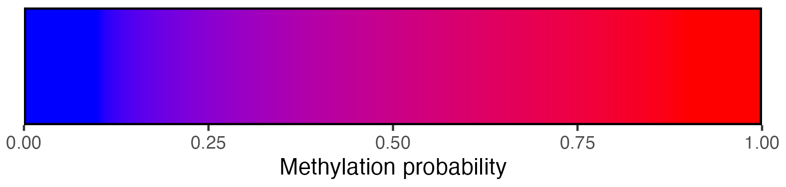
3 Loading data
3.1 Introduction to example_many_sequences
ggDNAvis comes with example dataset example_many_sequences. In this data, each row/observation represents one read. Reads are associated with metadata such as the participant and family to which they belong, and with sequence data such as the DNA sequence, FASTQ quality scores, and modification information retrieved from the MM and ML tags in a SAM/BAM file.
## View the first 4 rows of example_many_sequences data
print_table(head(example_many_sequences, 4))| family | individual | read | sequence | sequence_length | quality | methylation_locations | methylation_probabilities | hydroxymethylation_locations | hydroxymethylation_probabilities |
|---|---|---|---|---|---|---|---|---|---|
Family 1 |
F1-1 |
F1-1a |
GGCGGCGGCGGCGGCGGCGGCGGCGGCGGAGGAGGCGGCGGCGGAGGAGGCGGCGGCGGAGGAGGCGGCGGCGGAGGAGGCGGCGGCGGAGGAGGCGGCGGA |
102 |
)8@!9:/0/,0+-6?40,-I601:.';+5,@0.0%)!(20C*,2++*(00#/*+3;E-E)<I5.5G*CB8501;I3'.8233'3><:13)48F?09*>?I90 |
3,6,9,12,15,18,21,24,27,36,39,42,51,54,57,66,69,72,81,84,87,96,99 |
29,159,155,159,220,163,2,59,170,131,177,139,72,235,75,214,73,68,48,59,81,77,41 |
3,6,9,12,15,18,21,24,27,36,39,42,51,54,57,66,69,72,81,84,87,96,99 |
26,60,61,60,30,59,2,46,57,64,54,63,52,18,53,34,52,50,39,46,55,54,34 |
Family 1 |
F1-1 |
F1-1b |
GGCGGCGGCGGCGGCGGCGGCGGCGGCGGCGGCGGAGGAGGCGGCGGCGGAGGAGGCGGCGGA |
63 |
60-7,7943/*=5=)7<53-I=G6/&/7?8)<$12">/2C;4:9F8:816E,6C3*,1-2139 |
3,6,9,12,15,18,21,24,27,30,33,42,45,48,57,60 |
10,56,207,134,233,212,12,116,68,78,129,46,194,51,66,253 |
3,6,9,12,15,18,21,24,27,30,33,42,45,48,57,60 |
10,44,39,64,20,36,11,63,50,54,64,38,46,41,49,2 |
Family 1 |
F1-1 |
F1-1c |
GGCGGCGGCGGCGGCGGCGGCGGCGGCGGAGGAGGCGGCGGCGGAGGAGGCGGCGGCGGAGGAGGCGGCGGCGGAGGAGGCGGCGGA |
87 |
;F42DF52#C-*I75!4?9>IA0<30!-:I:;+7!:<7<8=G@5*91D%193/2;><IA8.I<.722,68*!25;69*<<8C9889@ |
3,6,9,12,15,18,21,24,27,36,39,42,51,54,57,66,69,72,81,84 |
206,141,165,80,159,84,128,173,124,62,195,19,79,183,129,39,129,126,192,45 |
3,6,9,12,15,18,21,24,27,36,39,42,51,54,57,66,69,72,81,84 |
40,63,58,55,60,56,64,56,64,47,46,17,55,52,64,33,63,64,47,37 |
Family 1 |
F1-1 |
F1-1d |
GGCGGCGGCGGCGGCGGCGGCGGCGGCGGCGGCGGCGGAGGAGGCGGCGGCGGAGGAGGCGGCGGCGGAGGAGGCGGCGGA |
81 |
:<*1D)89?27#8.3)9<2G<>I.=?58+:.=-8-3%6?7#/FG)198/+3?5/0E1=D9150A4D//650%5.@+@/8>0 |
3,6,9,12,15,18,21,24,27,30,33,36,45,48,51,60,63,66,75,78 |
216,221,11,81,4,61,180,79,130,13,144,31,228,4,200,23,132,98,18,82 |
3,6,9,12,15,18,21,24,27,30,33,36,45,48,51,60,63,66,75,78 |
33,29,10,55,3,46,53,54,64,12,63,27,24,4,43,21,64,60,17,55 |
The DNA sequence in column sequence is the information used for visualising single/multiple sequences. For visualising DNA modification, this data contains information on both 5-cytosine-methylation and 5-cytosine-hydroxymethylation. For a given modification type (e.g. methylation), visualisation requires a column of locations and a column of probabilities. In this dataset, the relevant columns are methylation_locations and methylation_probabilities for methylation and hydroxymethylation_locations and hydroxymethylation_probabilities for hydroxymethylation.
Locations are stored as a comma-condensed string of integers for each read, produced via vector_to_string(), and indicate the indices along the read at which the probability of modification was assessed. For example, methylation might be assessed at each CpG site, which in the read "GGCGGCGGAGGCGGCGGA" would be the third, sixth, twelfth, and fifteenth bases, thus the location string would be "3,6,12,15" for that read.
Probabilities are also a comma-condensed string of integers produced via vector_to_string(), but here each integer represents the probability that the corresponding base is modified. Probabilities are stored as 8-bit integers (0-255) where a score of p represents the probability space from \frac{p}{256} to \frac{p+1}{256}. For the read above, a probability string of "250,3,50,127" would indicate that the third base is almost certainly methylated (97.66%-98.05%), the sixth base is almost certainly not methylated (1.17%-1.56%), the twelfth base is most likely not methylated (19.53%-19.92%), and the fifteenth base may or may not be methylated (49.61%-50.00%)
## Function to convert integer scores to corresponding percentages
convert_8bit_to_decimal_prob <- function(x) {
    return(c(  x   / 256,
             (x+1) / 256))
}

## Convert comma-condensed string back to numerical vector
## string_to_vector() and vector_to_string() are crucial ggDNAvis helpers
probabilities <- string_to_vector("250,3,50,127")

## For each probability, print 8-bit score then percentage range
for (probability in probabilities) {
    percentages <- round(convert_8bit_to_decimal_prob(probability), 4) * 100
    cat("8-bit probability: ", probability, "\n", sep = "")
    cat("Decimal probability: ", percentages[1], "% - ", percentages[2], "%", "\n\n", sep = "")
}3.2 Introduction to string_to_vector() and vector_to_string()
Lots of the data used in ggDNAvis requires a series of multiple values to be stored within a single observation in a dataframe. The solution used here is condensing vectors to a single string (character value) for simple storage, then reconstituting the original vectors when needed. These functions are basic wrappers around strsplit() and paste(, collapse = ",") but are easy to use and readable.
Additionally, these can be used when reading SAM/BAM MM and ML tags, which are stored as comma-separated lists within modified FASTQ files, so can also be processed using these functions.
vector_to_string(c(1, 2, 3, 4))
string_to_vector("1,2,3,4") # the default vector type is numeric
vector_to_string(c("these", "are", "some", "words"))
string_to_vector("these,are,some,words", type = "character")
vector_to_string(c(TRUE, FALSE, TRUE))
string_to_vector("TRUE,FALSE,TRUE", type = "logical")If multiple strings (i.e. a character vector) are input to string_to_vector(), it will concatenate them and produce a single output vector. This is intended, useful behaviour to help with some of the visualisation code in this package. If a list of separate vectors for each input value is desired, lapply() can be used.
string_to_vector(c("1,2,3", "4,5,6"))3.3 Loading from FASTQ and metadata file
3.3.1 Standard FASTQ
To read in a normal FASTQ file (containing a read ID/header, sequence, and quality scores for each read), the function read_fastq() can be used. The example data file for this is inst/extdata/example_many_sequences_raw.fastq, accessible via system.file("extdata/example_many_sequences_raw.fastq", package = "ggDNAvis"):
## Look at first 16 lines of FASTQ
fastq_raw <- readLines(system.file("extdata/example_many_sequences_raw.fastq", package = "ggDNAvis"))
for (i in 1:16) {
    cat(fastq_raw[i], "\n")
}
## F1-1a
## GGCGGCGGCGGCGGCGGCGGCGGCGGCGGAGGAGGCGGCGGCGGAGGAGGCGGCGGCGGAGGAGGCGGCGGCGGAGGAGGCGGCGGCGGAGGAGGCGGCGGA
## +
## )8@!9:/0/,0+-6?40,-I601:.';+5,@0.0%)!(20C*,2++*(00#/*+3;E-E)<I5.5G*CB8501;I3'.8233'3><:13)48F?09*>?I90
## F1-1b
## GGCGGCGGCGGCGGCGGCGGCGGCGGCGGCGGCGGAGGAGGCGGCGGCGGAGGAGGCGGCGGA
## +
## 60-7,7943/*=5=)7<53-I=G6/&/7?8)<$12">/2C;4:9F8:816E,6C3*,1-2139
## F1-1c
## TCCGCCGCCTCCTCCGCCGCCGCCTCCTCCGCCGCCGCCTCCTCCGCCGCCGCCTCCTCCGCCGCCGCCGCCGCCGCCGCCGCCGCC
## +
## @9889C8<<*96;52!*86,227.<I.8AI<>;2/391%D19*5@G=8<7<:!7+;:I:-!03<0AI>9?4!57I*-C#25FD24F;
## F1-1d
## GGCGGCGGCGGCGGCGGCGGCGGCGGCGGCGGCGGCGGAGGAGGCGGCGGCGGAGGAGGCGGCGGCGGAGGAGGCGGCGGA
## +
## :<*1D)89?27#8.3)9<2G<>I.=?58+:.=-8-3%6?7#/FG)198/+3?5/0E1=D9150A4D//650%5.@+@/8>0
## Load data from FASTQ
fastq_data <- read_fastq(
    system.file("extdata/example_many_sequences_raw.fastq", package = "ggDNAvis"),
    calculate_length = TRUE,
    strip_at = TRUE
)

## View first 4 rows
print_table(head(fastq_data, 4))| read | sequence | quality | sequence_length |
|---|---|---|---|
F1-1a |
GGCGGCGGCGGCGGCGGCGGCGGCGGCGGAGGAGGCGGCGGCGGAGGAGGCGGCGGCGGAGGAGGCGGCGGCGGAGGAGGCGGCGGCGGAGGAGGCGGCGGA |
)8@!9:/0/,0+-6?40,-I601:.';+5,@0.0%)!(20C*,2++*(00#/*+3;E-E)<I5.5G*CB8501;I3'.8233'3><:13)48F?09*>?I90 |
102 |
F1-1b |
GGCGGCGGCGGCGGCGGCGGCGGCGGCGGCGGCGGAGGAGGCGGCGGCGGAGGAGGCGGCGGA |
60-7,7943/*=5=)7<53-I=G6/&/7?8)<$12">/2C;4:9F8:816E,6C3*,1-2139 |
63 |
F1-1c |
TCCGCCGCCTCCTCCGCCGCCGCCTCCTCCGCCGCCGCCTCCTCCGCCGCCGCCTCCTCCGCCGCCGCCGCCGCCGCCGCCGCCGCC |
@9889C8<<*96;52!*86,227.<I.8AI<>;2/391%D19*5@G=8<7<:!7+;:I:-!03<0AI>9?4!57I*-C#25FD24F; |
87 |
F1-1d |
GGCGGCGGCGGCGGCGGCGGCGGCGGCGGCGGCGGCGGAGGAGGCGGCGGCGGAGGAGGCGGCGGCGGAGGAGGCGGCGGA |
:<*1D)89?27#8.3)9<2G<>I.=?58+:.=-8-3%6?7#/FG)198/+3?5/0E1=D9150A4D//650%5.@+@/8>0 |
81 |
Using the basic read_fastq() function returns a dataframe with read ID, sequence, and quality columns. Optionally, a sequence_length column can be generated by setting calculate_length = TRUE. However, we can see that some of the sequences (e.g. F1-1c) are reversed. This occurs when the read is of the - strand at the biochemical level.
To convert reverse reads to their forward equivalents, and incorporate additional data such as the participant and family to which each read belongs, we will make use of a metadata file located at inst/extdata/example_many_sequences_metadata.csv.
Depending on how the FASTQ was created, the read IDs may be prefixed with @ (e.g. samtools fastq generally leaves these @s). This can cause issues with metadata merging if the FASTQ has @ at the start of each read ID but the metadata doesn’t, as then the reads can’t be matched up. The strip_at argument in read_fastq() and read_modified_fastq() (on by default), removes a single leading @ from each read ID that starts with @, and does nothing to read IDs that don’t start with @. If the metadata does have IDs beginning with @, then they can be kept in the FASTQ data by setting strip_at = FALSE.
## Load metadata from CSV
metadata <- read.csv(system.file("extdata/example_many_sequences_metadata.csv", package = "ggDNAvis"))

## View first 4 rows
print_table(head(metadata, 4))| family | individual | read | direction |
|---|---|---|---|
Family 1 |
F1-1 |
F1-1a |
forward |
Family 1 |
F1-1 |
F1-1b |
forward |
Family 1 |
F1-1 |
F1-1c |
reverse |
Family 1 |
F1-1 |
F1-1d |
forward |
We see that this metadata file contains the same read column with the same unique read IDs and a direction column specifying whether each read is "forward" or "reverse". These two columns are mandatory. Additionally, we have family and participant ID columns providing additional information on each read.
Note: the direction column can be produced manually. However, for large data volumes it may be more effective to use SAMtools to write TXT files of all forward and reverse read IDs via the -F/-f 16 flags, e.g.:
## bash/shell code for using SAMtools on the command line:

## See the samtools flag documentation for more details on why
## -F 16 selects forward reads and -f 16 selects reverse reads
samtools view -F 16 ${input_bam_file} | \
awk '{print $1}' > "forward_reads.txt"

samtools view -f 16 ${input_bam_file} | \
awk '{print $1}' > "reverse_reads.txt"
Then simply read the lines from each file and use that to assign directions:
## Use files from last step to construct vectors of forward and reverse IDs
forward_reads <- readLines("forward_reads.txt")
reverse_reads <- readLines("reverse_reads.txt")

## Use rep() to add a direction column
constructed_metadata <- data.frame(
    read = c(forward_reads, reverse_reads),
    direction = c(rep("forward", length(forward_reads)),
                  rep("reverse", length(reverse_reads)))
)
In any case, once we have metadata with the read and direction columns, we can use merge_fastq_with_metadata() to combine the metadata and the fastq data. Crucially, this function uses the direction column of the metadata to determine which reads are reverse, and reverse-complements these reverse reads only to produce a new column containing the forward version of all reads.
Note that there are three options for how to manage these reverse reads:
-
reverse_complement_mode = "DNA"reverse-complements, with A being mapped to T. This is the default. -
reverse_complement_mode = "RNA"reverse-complements, with A being mapped to U. -
reverse_complement_mode = "reverse_only"reverses but does not complement, meaning reverse reads will be shown 3’-5’ (i.e. complementary to the 5’-3’ forward reads) as opposed to being complemented into the 5’-3’ forward reads.
This example with proceed with the default reverse_complement_mode = "DNA", but be aware that "reverse_only" is an option if reverse reads want to be visualised aligned with forward reads without complementing.
## Merge fastq data with metadata
## This function reverse-complements reverse reads to get all forward versions
merged_fastq_data <- merge_fastq_with_metadata(fastq_data, metadata)

## View first 4 rows
print_table(head(merged_fastq_data, 4))| read | family | individual | direction | sequence | quality | sequence_length | forward_sequence | forward_quality |
|---|---|---|---|---|---|---|---|---|
F1-1a |
Family 1 |
F1-1 |
forward |
GGCGGCGGCGGCGGCGGCGGCGGCGGCGGAGGAGGCGGCGGCGGAGGAGGCGGCGGCGGAGGAGGCGGCGGCGGAGGAGGCGGCGGCGGAGGAGGCGGCGGA |
)8@!9:/0/,0+-6?40,-I601:.';+5,@0.0%)!(20C*,2++*(00#/*+3;E-E)<I5.5G*CB8501;I3'.8233'3><:13)48F?09*>?I90 |
102 |
GGCGGCGGCGGCGGCGGCGGCGGCGGCGGAGGAGGCGGCGGCGGAGGAGGCGGCGGCGGAGGAGGCGGCGGCGGAGGAGGCGGCGGCGGAGGAGGCGGCGGA |
)8@!9:/0/,0+-6?40,-I601:.';+5,@0.0%)!(20C*,2++*(00#/*+3;E-E)<I5.5G*CB8501;I3'.8233'3><:13)48F?09*>?I90 |
F1-1b |
Family 1 |
F1-1 |
forward |
GGCGGCGGCGGCGGCGGCGGCGGCGGCGGCGGCGGAGGAGGCGGCGGCGGAGGAGGCGGCGGA |
60-7,7943/*=5=)7<53-I=G6/&/7?8)<$12">/2C;4:9F8:816E,6C3*,1-2139 |
63 |
GGCGGCGGCGGCGGCGGCGGCGGCGGCGGCGGCGGAGGAGGCGGCGGCGGAGGAGGCGGCGGA |
60-7,7943/*=5=)7<53-I=G6/&/7?8)<$12">/2C;4:9F8:816E,6C3*,1-2139 |
F1-1c |
Family 1 |
F1-1 |
reverse |
TCCGCCGCCTCCTCCGCCGCCGCCTCCTCCGCCGCCGCCTCCTCCGCCGCCGCCTCCTCCGCCGCCGCCGCCGCCGCCGCCGCCGCC |
@9889C8<<*96;52!*86,227.<I.8AI<>;2/391%D19*5@G=8<7<:!7+;:I:-!03<0AI>9?4!57I*-C#25FD24F; |
87 |
GGCGGCGGCGGCGGCGGCGGCGGCGGCGGAGGAGGCGGCGGCGGAGGAGGCGGCGGCGGAGGAGGCGGCGGCGGAGGAGGCGGCGGA |
;F42DF52#C-*I75!4?9>IA0<30!-:I:;+7!:<7<8=G@5*91D%193/2;><IA8.I<.722,68*!25;69*<<8C9889@ |
F1-1d |
Family 1 |
F1-1 |
forward |
GGCGGCGGCGGCGGCGGCGGCGGCGGCGGCGGCGGCGGAGGAGGCGGCGGCGGAGGAGGCGGCGGCGGAGGAGGCGGCGGA |
:<*1D)89?27#8.3)9<2G<>I.=?58+:.=-8-3%6?7#/FG)198/+3?5/0E1=D9150A4D//650%5.@+@/8>0 |
81 |
GGCGGCGGCGGCGGCGGCGGCGGCGGCGGCGGCGGCGGAGGAGGCGGCGGCGGAGGAGGCGGCGGCGGAGGAGGCGGCGGA |
:<*1D)89?27#8.3)9<2G<>I.=?58+:.=-8-3%6?7#/FG)198/+3?5/0E1=D9150A4D//650%5.@+@/8>0 |
Now we have a forward_sequence column (scroll to the right if you can’t see it!). We can now reformat this data to be exactly the same as the included example_many_sequences data:
## Subset to only the columns present in example_many_sequences
merged_fastq_data <- merged_fastq_data[, c("family", "individual", "read", "forward_sequence", "sequence_length", "forward_quality")]

## Rename "forward_sequence" to "sequence" and same for quality
colnames(merged_fastq_data)[c(4,6)] <- c("sequence", "quality")

## View first 4 rows of data produced from files
print_table(head(merged_fastq_data, 4))| family | individual | read | sequence | sequence_length | quality |
|---|---|---|---|---|---|
Family 1 |
F1-1 |
F1-1a |
GGCGGCGGCGGCGGCGGCGGCGGCGGCGGAGGAGGCGGCGGCGGAGGAGGCGGCGGCGGAGGAGGCGGCGGCGGAGGAGGCGGCGGCGGAGGAGGCGGCGGA |
102 |
)8@!9:/0/,0+-6?40,-I601:.';+5,@0.0%)!(20C*,2++*(00#/*+3;E-E)<I5.5G*CB8501;I3'.8233'3><:13)48F?09*>?I90 |
Family 1 |
F1-1 |
F1-1b |
GGCGGCGGCGGCGGCGGCGGCGGCGGCGGCGGCGGAGGAGGCGGCGGCGGAGGAGGCGGCGGA |
63 |
60-7,7943/*=5=)7<53-I=G6/&/7?8)<$12">/2C;4:9F8:816E,6C3*,1-2139 |
Family 1 |
F1-1 |
F1-1c |
GGCGGCGGCGGCGGCGGCGGCGGCGGCGGAGGAGGCGGCGGCGGAGGAGGCGGCGGCGGAGGAGGCGGCGGCGGAGGAGGCGGCGGA |
87 |
;F42DF52#C-*I75!4?9>IA0<30!-:I:;+7!:<7<8=G@5*91D%193/2;><IA8.I<.722,68*!25;69*<<8C9889@ |
Family 1 |
F1-1 |
F1-1d |
GGCGGCGGCGGCGGCGGCGGCGGCGGCGGCGGCGGCGGAGGAGGCGGCGGCGGAGGAGGCGGCGGCGGAGGAGGCGGCGGA |
81 |
:<*1D)89?27#8.3)9<2G<>I.=?58+:.=-8-3%6?7#/FG)198/+3?5/0E1=D9150A4D//650%5.@+@/8>0 |
## View first 4 rows of example_many_sequences (with modification columns excluded)
print_table(head(example_many_sequences[, 1:6], 4))| family | individual | read | sequence | sequence_length | quality |
|---|---|---|---|---|---|
Family 1 |
F1-1 |
F1-1a |
GGCGGCGGCGGCGGCGGCGGCGGCGGCGGAGGAGGCGGCGGCGGAGGAGGCGGCGGCGGAGGAGGCGGCGGCGGAGGAGGCGGCGGCGGAGGAGGCGGCGGA |
102 |
)8@!9:/0/,0+-6?40,-I601:.';+5,@0.0%)!(20C*,2++*(00#/*+3;E-E)<I5.5G*CB8501;I3'.8233'3><:13)48F?09*>?I90 |
Family 1 |
F1-1 |
F1-1b |
GGCGGCGGCGGCGGCGGCGGCGGCGGCGGCGGCGGAGGAGGCGGCGGCGGAGGAGGCGGCGGA |
63 |
60-7,7943/*=5=)7<53-I=G6/&/7?8)<$12">/2C;4:9F8:816E,6C3*,1-2139 |
Family 1 |
F1-1 |
F1-1c |
GGCGGCGGCGGCGGCGGCGGCGGCGGCGGAGGAGGCGGCGGCGGAGGAGGCGGCGGCGGAGGAGGCGGCGGCGGAGGAGGCGGCGGA |
87 |
;F42DF52#C-*I75!4?9>IA0<30!-:I:;+7!:<7<8=G@5*91D%193/2;><IA8.I<.722,68*!25;69*<<8C9889@ |
Family 1 |
F1-1 |
F1-1d |
GGCGGCGGCGGCGGCGGCGGCGGCGGCGGCGGCGGCGGAGGAGGCGGCGGCGGAGGAGGCGGCGGCGGAGGAGGCGGCGGA |
81 |
:<*1D)89?27#8.3)9<2G<>I.=?58+:.=-8-3%6?7#/FG)198/+3?5/0E1=D9150A4D//650%5.@+@/8>0 |
## Check if equal
identical(merged_fastq_data, example_many_sequences[, 1:6])So, from just a standard FASTQ file and a simple metadata CSV we have successfully reproduced the example_many_sequences data (excluding methylation/modification information) via read_fastq() and merge_fastq_with_metadata(). We can also write from this dataframe to FASTQ using write_fastq():
## Use write_fastq with filename = NA and return = TRUE to create the FASTQ,
## but return it as a character vector rather than writing to file.
output_fastq <- write_fastq(
    merged_fastq_data,
    filename = NA,
    return = TRUE,
    read_id_colname = "read",
    sequence_colname = "sequence",
    quality_colname = "quality"
)

## View first 16 lines
for (i in 1:16) {
    cat(output_fastq[i], "\n")
}
## F1-1a
## GGCGGCGGCGGCGGCGGCGGCGGCGGCGGAGGAGGCGGCGGCGGAGGAGGCGGCGGCGGAGGAGGCGGCGGCGGAGGAGGCGGCGGCGGAGGAGGCGGCGGA
## +
## )8@!9:/0/,0+-6?40,-I601:.';+5,@0.0%)!(20C*,2++*(00#/*+3;E-E)<I5.5G*CB8501;I3'.8233'3><:13)48F?09*>?I90
## F1-1b
## GGCGGCGGCGGCGGCGGCGGCGGCGGCGGCGGCGGAGGAGGCGGCGGCGGAGGAGGCGGCGGA
## +
## 60-7,7943/*=5=)7<53-I=G6/&/7?8)<$12">/2C;4:9F8:816E,6C3*,1-2139
## F1-1c
## GGCGGCGGCGGCGGCGGCGGCGGCGGCGGAGGAGGCGGCGGCGGAGGAGGCGGCGGCGGAGGAGGCGGCGGCGGAGGAGGCGGCGGA
## +
## ;F42DF52#C-*I75!4?9>IA0<30!-:I:;+7!:<7<8=G@5*91D%193/2;><IA8.I<.722,68*!25;69*<<8C9889@
## F1-1d
## GGCGGCGGCGGCGGCGGCGGCGGCGGCGGCGGCGGCGGAGGAGGCGGCGGCGGAGGAGGCGGCGGCGGAGGAGGCGGCGGA
## +
## :<*1D)89?27#8.3)9<2G<>I.=?58+:.=-8-3%6?7#/FG)198/+3?5/0E1=D9150A4D//650%5.@+@/8>0Note that this is not quite identical to the original. That’s because we wrote from the forward-sequence and forward-quality columns (after renaming), so the new FASTQ contains all forward versions. If we wanted the original FASTQ we would just provide colnames for the original sequence and quality rather than the forward versions.
Do be careful that either both sequence and quality are the forward versions or neither are. If they are mismatched then the new FASTQ will be wrong.
3.3.2 Modified FASTQ (eg methylation)
FASTQ files can be modified to include DNA modification (most often 5-cytosine-methylation) information within the header lines. This is a very specific file format that is generally produced under the following conditions:
- Oxford Nanopore sequencing is used
- Raw FAST5/POD5/BLOW5 signal files are basecalled to SAM/BAM using a modification-capable model in Guppy or Dorado (see modified basecalling documentation)
- SAM/BAM, which stores modification information in the MM and ML tags, is converted to FASTQ with MM/ML information copied to header rows via:
ggDNAvis then contains tools for reading from, processing, and writing to these modified FASTQ files. The example data file for this is inst/extdata/example_many_sequences_raw_modified.fastq, accessible via system.file("extdata/example_many_sequences_raw_modified.fastq", package = "ggDNAvis"):
## Look at first 16 lines of FASTQ
modified_fastq_raw <- readLines(system.file("extdata/example_many_sequences_raw_modified.fastq", package = "ggDNAvis"))
for (i in 1:16) {
    cat(modified_fastq_raw[i], "\n")
}
## F1-1a MM:Z:C+h?,0,0,0,0,0,0,0,0,0,0,0,0,0,0,0,0,0,0,0,0,0,0,0;C+m?,0,0,0,0,0,0,0,0,0,0,0,0,0,0,0,0,0,0,0,0,0,0,0; ML:B:C,26,60,61,60,30,59,2,46,57,64,54,63,52,18,53,34,52,50,39,46,55,54,34,29,159,155,159,220,163,2,59,170,131,177,139,72,235,75,214,73,68,48,59,81,77,41
## GGCGGCGGCGGCGGCGGCGGCGGCGGCGGAGGAGGCGGCGGCGGAGGAGGCGGCGGCGGAGGAGGCGGCGGCGGAGGAGGCGGCGGCGGAGGAGGCGGCGGA
## +
## )8@!9:/0/,0+-6?40,-I601:.';+5,@0.0%)!(20C*,2++*(00#/*+3;E-E)<I5.5G*CB8501;I3'.8233'3><:13)48F?09*>?I90
## F1-1b MM:Z:C+h?,0,0,0,0,0,0,0,0,0,0,0,0,0,0,0,0;C+m?,0,0,0,0,0,0,0,0,0,0,0,0,0,0,0,0; ML:B:C,10,44,39,64,20,36,11,63,50,54,64,38,46,41,49,2,10,56,207,134,233,212,12,116,68,78,129,46,194,51,66,253
## GGCGGCGGCGGCGGCGGCGGCGGCGGCGGCGGCGGAGGAGGCGGCGGCGGAGGAGGCGGCGGA
## +
## 60-7,7943/*=5=)7<53-I=G6/&/7?8)<$12">/2C;4:9F8:816E,6C3*,1-2139
## F1-1c MM:Z:C+h?,1,1,5,1,1,5,1,1,5,1,1,5,1,1,1,1,1,1,1,1;C+m?,1,1,5,1,1,5,1,1,5,1,1,5,1,1,1,1,1,1,1,1; ML:B:C,37,47,64,63,33,64,52,55,17,46,47,64,56,64,56,60,55,58,63,40,45,192,126,129,39,129,183,79,19,195,62,124,173,128,84,159,80,165,141,206
## TCCGCCGCCTCCTCCGCCGCCGCCTCCTCCGCCGCCGCCTCCTCCGCCGCCGCCTCCTCCGCCGCCGCCGCCGCCGCCGCCGCCGCC
## +
## @9889C8<<*96;52!*86,227.<I.8AI<>;2/391%D19*5@G=8<7<:!7+;:I:-!03<0AI>9?4!57I*-C#25FD24F;
## F1-1d MM:Z:C+h?,0,0,0,0,0,0,0,0,0,0,0,0,0,0,0,0,0,0,0,0;C+m?,0,0,0,0,0,0,0,0,0,0,0,0,0,0,0,0,0,0,0,0; ML:B:C,33,29,10,55,3,46,53,54,64,12,63,27,24,4,43,21,64,60,17,55,216,221,11,81,4,61,180,79,130,13,144,31,228,4,200,23,132,98,18,82
## GGCGGCGGCGGCGGCGGCGGCGGCGGCGGCGGCGGCGGAGGAGGCGGCGGCGGAGGAGGCGGCGGCGGAGGAGGCGGCGGA
## +
## :<*1D)89?27#8.3)9<2G<>I.=?58+:.=-8-3%6?7#/FG)198/+3?5/0E1=D9150A4D//650%5.@+@/8>0This file is identical to the standard FASTQ seen in the reading standard FASTQ section in the sequence and quality lines, but has the MM and ML tags stored in the header. See the SAM tags specification or the documentation for read_modified_fastq(), merge_methylation_with_metadata(), and reverse_locations_if_needed() for a comprehensive explanation of how these store methylation/modification information.
The modification information stored in these FASTQ header lines can be parsed with read_modified_fastq(). This converts the locations from the SAM/BAM MM format to simply being the indices along the read at which modification was assessed (starting indexing at 1). For example, in F1-1a, the C+m? (methylation) locations start "3,6,9,12", indicating that the third, sixth, ninth, and twelfth bases in the read were assessed for probability of methylation. Checking the sequence, we see that all of these are CpG sites (CG dinucleotides), which are the main DNA methylation sites in the genome. For each assessed site, the modification probability is given as an 8-bit integer (0-255), where 0 represents ~0% modification probability and 255 represents ~100% modification probability (this is fully explained in introduction to example_many_sequences).
## Load data from FASTQ
methylation_data <- read_modified_fastq(
    system.file("extdata/example_many_sequences_raw_modified.fastq", package = "ggDNAvis"),
    strip_at = TRUE
)

## View first 4 rows
print_table(head(methylation_data, 4))| read | sequence | sequence_length | quality | modification_types | C+h?_locations | C+h?_probabilities | C+m?_locations | C+m?_probabilities |
|---|---|---|---|---|---|---|---|---|
F1-1a |
GGCGGCGGCGGCGGCGGCGGCGGCGGCGGAGGAGGCGGCGGCGGAGGAGGCGGCGGCGGAGGAGGCGGCGGCGGAGGAGGCGGCGGCGGAGGAGGCGGCGGA |
102 |
)8@!9:/0/,0+-6?40,-I601:.';+5,@0.0%)!(20C*,2++*(00#/*+3;E-E)<I5.5G*CB8501;I3'.8233'3><:13)48F?09*>?I90 |
C+h?,C+m? |
3,6,9,12,15,18,21,24,27,36,39,42,51,54,57,66,69,72,81,84,87,96,99 |
26,60,61,60,30,59,2,46,57,64,54,63,52,18,53,34,52,50,39,46,55,54,34 |
3,6,9,12,15,18,21,24,27,36,39,42,51,54,57,66,69,72,81,84,87,96,99 |
29,159,155,159,220,163,2,59,170,131,177,139,72,235,75,214,73,68,48,59,81,77,41 |
F1-1b |
GGCGGCGGCGGCGGCGGCGGCGGCGGCGGCGGCGGAGGAGGCGGCGGCGGAGGAGGCGGCGGA |
63 |
60-7,7943/*=5=)7<53-I=G6/&/7?8)<$12">/2C;4:9F8:816E,6C3*,1-2139 |
C+h?,C+m? |
3,6,9,12,15,18,21,24,27,30,33,42,45,48,57,60 |
10,44,39,64,20,36,11,63,50,54,64,38,46,41,49,2 |
3,6,9,12,15,18,21,24,27,30,33,42,45,48,57,60 |
10,56,207,134,233,212,12,116,68,78,129,46,194,51,66,253 |
F1-1c |
TCCGCCGCCTCCTCCGCCGCCGCCTCCTCCGCCGCCGCCTCCTCCGCCGCCGCCTCCTCCGCCGCCGCCGCCGCCGCCGCCGCCGCC |
87 |
@9889C8<<*96;52!*86,227.<I.8AI<>;2/391%D19*5@G=8<7<:!7+;:I:-!03<0AI>9?4!57I*-C#25FD24F; |
C+h?,C+m? |
3,6,15,18,21,30,33,36,45,48,51,60,63,66,69,72,75,78,81,84 |
37,47,64,63,33,64,52,55,17,46,47,64,56,64,56,60,55,58,63,40 |
3,6,15,18,21,30,33,36,45,48,51,60,63,66,69,72,75,78,81,84 |
45,192,126,129,39,129,183,79,19,195,62,124,173,128,84,159,80,165,141,206 |
F1-1d |
GGCGGCGGCGGCGGCGGCGGCGGCGGCGGCGGCGGCGGAGGAGGCGGCGGCGGAGGAGGCGGCGGCGGAGGAGGCGGCGGA |
81 |
:<*1D)89?27#8.3)9<2G<>I.=?58+:.=-8-3%6?7#/FG)198/+3?5/0E1=D9150A4D//650%5.@+@/8>0 |
C+h?,C+m? |
3,6,9,12,15,18,21,24,27,30,33,36,45,48,51,60,63,66,75,78 |
33,29,10,55,3,46,53,54,64,12,63,27,24,4,43,21,64,60,17,55 |
3,6,9,12,15,18,21,24,27,30,33,36,45,48,51,60,63,66,75,78 |
216,221,11,81,4,61,180,79,130,13,144,31,228,4,200,23,132,98,18,82 |
Ultimately, read_modified_fastq() outputs a dataframe with the standard read information (ID, sequence, length, quality), a column stating which modification types were assessed for each read (e.g. "C+h?" for hydroxymethylation or "C+m?" for methylation - refer to the SAM tags specification), and for each modification type, a column of assessed locations (indices along the read) and a column of modification probabilities (as 8-bit integers).
Modification types, locations, and probabilities are all stored as comma-condensed strings produced from vectors via vector_to_string(). These can be converted back to vectors via string_to_vector() - see introduction to string/vector functions.
As with the standard FASTQ, some of the reads in the modified FASTQ are reverse. However, as the assessed modification locations are indices along the read and the probabilities correspond to locations in sequence, the modification information needs to be reversed in addition to reverse complementing the DNA sequence. Analogous to before, this is achieved via the merge_methylation_with_metadata() function.
## Load metadata from CSV
metadata <- read.csv(system.file("extdata/example_many_sequences_metadata.csv", package = "ggDNAvis"))

## View first 4 rows
print_table(head(metadata, 4))| family | individual | read | direction |
|---|---|---|---|
Family 1 |
F1-1 |
F1-1a |
forward |
Family 1 |
F1-1 |
F1-1b |
forward |
Family 1 |
F1-1 |
F1-1c |
reverse |
Family 1 |
F1-1 |
F1-1d |
forward |
The metadata is identical to its previous use in the reading from standard FASTQ section.
## Merge fastq data with metadata
## This function reverse-complements reverse reads to get all forward versions
## And correctly flips location and probability information
## See ?merged_methylation_data and ?reverse_locations_if_needed for details
merged_methylation_data <- merge_methylation_with_metadata(methylation_data, metadata)

## View first 4 rows
print_table(head(merged_methylation_data, 4))| read | family | individual | direction | sequence | sequence_length | quality | modification_types | C+h?_locations | C+h?_probabilities | C+m?_locations | C+m?_probabilities | forward_sequence | forward_quality | forward_C+h?_locations | forward_C+h?_probabilities | forward_C+m?_locations | forward_C+m?_probabilities |
|---|---|---|---|---|---|---|---|---|---|---|---|---|---|---|---|---|---|
F1-1a |
Family 1 |
F1-1 |
forward |
GGCGGCGGCGGCGGCGGCGGCGGCGGCGGAGGAGGCGGCGGCGGAGGAGGCGGCGGCGGAGGAGGCGGCGGCGGAGGAGGCGGCGGCGGAGGAGGCGGCGGA |
102 |
)8@!9:/0/,0+-6?40,-I601:.';+5,@0.0%)!(20C*,2++*(00#/*+3;E-E)<I5.5G*CB8501;I3'.8233'3><:13)48F?09*>?I90 |
C+h?,C+m? |
3,6,9,12,15,18,21,24,27,36,39,42,51,54,57,66,69,72,81,84,87,96,99 |
26,60,61,60,30,59,2,46,57,64,54,63,52,18,53,34,52,50,39,46,55,54,34 |
3,6,9,12,15,18,21,24,27,36,39,42,51,54,57,66,69,72,81,84,87,96,99 |
29,159,155,159,220,163,2,59,170,131,177,139,72,235,75,214,73,68,48,59,81,77,41 |
GGCGGCGGCGGCGGCGGCGGCGGCGGCGGAGGAGGCGGCGGCGGAGGAGGCGGCGGCGGAGGAGGCGGCGGCGGAGGAGGCGGCGGCGGAGGAGGCGGCGGA |
)8@!9:/0/,0+-6?40,-I601:.';+5,@0.0%)!(20C*,2++*(00#/*+3;E-E)<I5.5G*CB8501;I3'.8233'3><:13)48F?09*>?I90 |
3,6,9,12,15,18,21,24,27,36,39,42,51,54,57,66,69,72,81,84,87,96,99 |
26,60,61,60,30,59,2,46,57,64,54,63,52,18,53,34,52,50,39,46,55,54,34 |
3,6,9,12,15,18,21,24,27,36,39,42,51,54,57,66,69,72,81,84,87,96,99 |
29,159,155,159,220,163,2,59,170,131,177,139,72,235,75,214,73,68,48,59,81,77,41 |
F1-1b |
Family 1 |
F1-1 |
forward |
GGCGGCGGCGGCGGCGGCGGCGGCGGCGGCGGCGGAGGAGGCGGCGGCGGAGGAGGCGGCGGA |
63 |
60-7,7943/*=5=)7<53-I=G6/&/7?8)<$12">/2C;4:9F8:816E,6C3*,1-2139 |
C+h?,C+m? |
3,6,9,12,15,18,21,24,27,30,33,42,45,48,57,60 |
10,44,39,64,20,36,11,63,50,54,64,38,46,41,49,2 |
3,6,9,12,15,18,21,24,27,30,33,42,45,48,57,60 |
10,56,207,134,233,212,12,116,68,78,129,46,194,51,66,253 |
GGCGGCGGCGGCGGCGGCGGCGGCGGCGGCGGCGGAGGAGGCGGCGGCGGAGGAGGCGGCGGA |
60-7,7943/*=5=)7<53-I=G6/&/7?8)<$12">/2C;4:9F8:816E,6C3*,1-2139 |
3,6,9,12,15,18,21,24,27,30,33,42,45,48,57,60 |
10,44,39,64,20,36,11,63,50,54,64,38,46,41,49,2 |
3,6,9,12,15,18,21,24,27,30,33,42,45,48,57,60 |
10,56,207,134,233,212,12,116,68,78,129,46,194,51,66,253 |
F1-1c |
Family 1 |
F1-1 |
reverse |
TCCGCCGCCTCCTCCGCCGCCGCCTCCTCCGCCGCCGCCTCCTCCGCCGCCGCCTCCTCCGCCGCCGCCGCCGCCGCCGCCGCCGCC |
87 |
@9889C8<<*96;52!*86,227.<I.8AI<>;2/391%D19*5@G=8<7<:!7+;:I:-!03<0AI>9?4!57I*-C#25FD24F; |
C+h?,C+m? |
3,6,15,18,21,30,33,36,45,48,51,60,63,66,69,72,75,78,81,84 |
37,47,64,63,33,64,52,55,17,46,47,64,56,64,56,60,55,58,63,40 |
3,6,15,18,21,30,33,36,45,48,51,60,63,66,69,72,75,78,81,84 |
45,192,126,129,39,129,183,79,19,195,62,124,173,128,84,159,80,165,141,206 |
GGCGGCGGCGGCGGCGGCGGCGGCGGCGGAGGAGGCGGCGGCGGAGGAGGCGGCGGCGGAGGAGGCGGCGGCGGAGGAGGCGGCGGA |
;F42DF52#C-*I75!4?9>IA0<30!-:I:;+7!:<7<8=G@5*91D%193/2;><IA8.I<.722,68*!25;69*<<8C9889@ |
4,7,10,13,16,19,22,25,28,37,40,43,52,55,58,67,70,73,82,85 |
40,63,58,55,60,56,64,56,64,47,46,17,55,52,64,33,63,64,47,37 |
4,7,10,13,16,19,22,25,28,37,40,43,52,55,58,67,70,73,82,85 |
206,141,165,80,159,84,128,173,124,62,195,19,79,183,129,39,129,126,192,45 |
F1-1d |
Family 1 |
F1-1 |
forward |
GGCGGCGGCGGCGGCGGCGGCGGCGGCGGCGGCGGCGGAGGAGGCGGCGGCGGAGGAGGCGGCGGCGGAGGAGGCGGCGGA |
81 |
:<*1D)89?27#8.3)9<2G<>I.=?58+:.=-8-3%6?7#/FG)198/+3?5/0E1=D9150A4D//650%5.@+@/8>0 |
C+h?,C+m? |
3,6,9,12,15,18,21,24,27,30,33,36,45,48,51,60,63,66,75,78 |
33,29,10,55,3,46,53,54,64,12,63,27,24,4,43,21,64,60,17,55 |
3,6,9,12,15,18,21,24,27,30,33,36,45,48,51,60,63,66,75,78 |
216,221,11,81,4,61,180,79,130,13,144,31,228,4,200,23,132,98,18,82 |
GGCGGCGGCGGCGGCGGCGGCGGCGGCGGCGGCGGCGGAGGAGGCGGCGGCGGAGGAGGCGGCGGCGGAGGAGGCGGCGGA |
:<*1D)89?27#8.3)9<2G<>I.=?58+:.=-8-3%6?7#/FG)198/+3?5/0E1=D9150A4D//650%5.@+@/8>0 |
3,6,9,12,15,18,21,24,27,30,33,36,45,48,51,60,63,66,75,78 |
33,29,10,55,3,46,53,54,64,12,63,27,24,4,43,21,64,60,17,55 |
3,6,9,12,15,18,21,24,27,30,33,36,45,48,51,60,63,66,75,78 |
216,221,11,81,4,61,180,79,130,13,144,31,228,4,200,23,132,98,18,82 |
The merged methylation data contains forward_ rows for sequence and quality, as before, but also for hydroxymethylation and methylation locations and probabilities. However, looking at the modification locations columns (scroll right on the table), we can see that the indices assessed for modification are 4, 7, 10 etc for sequence "GGCGGCGGCGGC...". This is because the actual biochemical modification was on the Cs on the reverse strand, corresponding to Gs on the forward strand according to Watson-Crick base pairing. For many purposes, it may be desirable to keep these positions to indicate that in reality, the modification occurred at exactly that location on the other strand. This is accomplished by setting offset = 0 (the default) inside merge_methylation_with_metadata().
However, there is also the option to offset the modification locations by 1. For symmetrical modification sites such as CGs, this means that when the C on the reverse strand is modified, that gets attributed to the C on the forward strand even though the direct complementary base is the G. The advantage of this is that it means CG sites (i.e. potential methylation sites) always have 5-methylcytosine modifications associated with the C of each CG, regardless of which strand the information came from. This is also often useful, as it ensures the information is consistent and (provided locations are palindromic when reverse-complemented) modifications are always attached to the correct base e.g. C-methylation to C. This is accomplished by setting offset = 1 inside merge_methylation_with_metadata().
Either of these options can be valid and useful, but make sure you think about it!
## Here the stars represent the true biochemical modifications on the reverse strand:
## (occurring at the Cs of CGs in the 5'-3' direction)
##
##
## 5'  GGCGGCGGCGGCGGCGGA  3'
## 3'  CCGCCGCCGCCGCCGCCT  5'
##        *  *  *  *  *

## If we take the complementary locations on the forward strand,
## the modification locations correspond to Gs rather than Cs,
## but are in the exact same locations:
##
##        o  o  o  o  o
## 5'  GGCGGCGGCGGCGGCGGA  3'
## 3'  CCGCCGCCGCCGCCGCCT  5'
##        *  *  *  *  *

## If we offset the locations by 1 on the forward strand,
## the modifications are always associated with the C of a CG,
## but the locations are moved slightly:
##
##       o  o  o  o  o
## 5'  GGCGGCGGCGGCGGCGGA  3'
## 3'  CCGCCGCCGCCGCCGCCT  5'
##        *  *  *  *  *
We will proceed with offset = 1 so that the forward versions match up with example_many_sequences.
## Merge fastq data with metadata, offsetting reversed locations by 1
merged_methylation_data <- merge_methylation_with_metadata(
    methylation_data,
    metadata,
    reversed_location_offset = 1
)

## View first 4 rows
print_table(head(merged_methylation_data, 4))| read | family | individual | direction | sequence | sequence_length | quality | modification_types | C+h?_locations | C+h?_probabilities | C+m?_locations | C+m?_probabilities | forward_sequence | forward_quality | forward_C+h?_locations | forward_C+h?_probabilities | forward_C+m?_locations | forward_C+m?_probabilities |
|---|---|---|---|---|---|---|---|---|---|---|---|---|---|---|---|---|---|
F1-1a |
Family 1 |
F1-1 |
forward |
GGCGGCGGCGGCGGCGGCGGCGGCGGCGGAGGAGGCGGCGGCGGAGGAGGCGGCGGCGGAGGAGGCGGCGGCGGAGGAGGCGGCGGCGGAGGAGGCGGCGGA |
102 |
)8@!9:/0/,0+-6?40,-I601:.';+5,@0.0%)!(20C*,2++*(00#/*+3;E-E)<I5.5G*CB8501;I3'.8233'3><:13)48F?09*>?I90 |
C+h?,C+m? |
3,6,9,12,15,18,21,24,27,36,39,42,51,54,57,66,69,72,81,84,87,96,99 |
26,60,61,60,30,59,2,46,57,64,54,63,52,18,53,34,52,50,39,46,55,54,34 |
3,6,9,12,15,18,21,24,27,36,39,42,51,54,57,66,69,72,81,84,87,96,99 |
29,159,155,159,220,163,2,59,170,131,177,139,72,235,75,214,73,68,48,59,81,77,41 |
GGCGGCGGCGGCGGCGGCGGCGGCGGCGGAGGAGGCGGCGGCGGAGGAGGCGGCGGCGGAGGAGGCGGCGGCGGAGGAGGCGGCGGCGGAGGAGGCGGCGGA |
)8@!9:/0/,0+-6?40,-I601:.';+5,@0.0%)!(20C*,2++*(00#/*+3;E-E)<I5.5G*CB8501;I3'.8233'3><:13)48F?09*>?I90 |
3,6,9,12,15,18,21,24,27,36,39,42,51,54,57,66,69,72,81,84,87,96,99 |
26,60,61,60,30,59,2,46,57,64,54,63,52,18,53,34,52,50,39,46,55,54,34 |
3,6,9,12,15,18,21,24,27,36,39,42,51,54,57,66,69,72,81,84,87,96,99 |
29,159,155,159,220,163,2,59,170,131,177,139,72,235,75,214,73,68,48,59,81,77,41 |
F1-1b |
Family 1 |
F1-1 |
forward |
GGCGGCGGCGGCGGCGGCGGCGGCGGCGGCGGCGGAGGAGGCGGCGGCGGAGGAGGCGGCGGA |
63 |
60-7,7943/*=5=)7<53-I=G6/&/7?8)<$12">/2C;4:9F8:816E,6C3*,1-2139 |
C+h?,C+m? |
3,6,9,12,15,18,21,24,27,30,33,42,45,48,57,60 |
10,44,39,64,20,36,11,63,50,54,64,38,46,41,49,2 |
3,6,9,12,15,18,21,24,27,30,33,42,45,48,57,60 |
10,56,207,134,233,212,12,116,68,78,129,46,194,51,66,253 |
GGCGGCGGCGGCGGCGGCGGCGGCGGCGGCGGCGGAGGAGGCGGCGGCGGAGGAGGCGGCGGA |
60-7,7943/*=5=)7<53-I=G6/&/7?8)<$12">/2C;4:9F8:816E,6C3*,1-2139 |
3,6,9,12,15,18,21,24,27,30,33,42,45,48,57,60 |
10,44,39,64,20,36,11,63,50,54,64,38,46,41,49,2 |
3,6,9,12,15,18,21,24,27,30,33,42,45,48,57,60 |
10,56,207,134,233,212,12,116,68,78,129,46,194,51,66,253 |
F1-1c |
Family 1 |
F1-1 |
reverse |
TCCGCCGCCTCCTCCGCCGCCGCCTCCTCCGCCGCCGCCTCCTCCGCCGCCGCCTCCTCCGCCGCCGCCGCCGCCGCCGCCGCCGCC |
87 |
@9889C8<<*96;52!*86,227.<I.8AI<>;2/391%D19*5@G=8<7<:!7+;:I:-!03<0AI>9?4!57I*-C#25FD24F; |
C+h?,C+m? |
3,6,15,18,21,30,33,36,45,48,51,60,63,66,69,72,75,78,81,84 |
37,47,64,63,33,64,52,55,17,46,47,64,56,64,56,60,55,58,63,40 |
3,6,15,18,21,30,33,36,45,48,51,60,63,66,69,72,75,78,81,84 |
45,192,126,129,39,129,183,79,19,195,62,124,173,128,84,159,80,165,141,206 |
GGCGGCGGCGGCGGCGGCGGCGGCGGCGGAGGAGGCGGCGGCGGAGGAGGCGGCGGCGGAGGAGGCGGCGGCGGAGGAGGCGGCGGA |
;F42DF52#C-*I75!4?9>IA0<30!-:I:;+7!:<7<8=G@5*91D%193/2;><IA8.I<.722,68*!25;69*<<8C9889@ |
3,6,9,12,15,18,21,24,27,36,39,42,51,54,57,66,69,72,81,84 |
40,63,58,55,60,56,64,56,64,47,46,17,55,52,64,33,63,64,47,37 |
3,6,9,12,15,18,21,24,27,36,39,42,51,54,57,66,69,72,81,84 |
206,141,165,80,159,84,128,173,124,62,195,19,79,183,129,39,129,126,192,45 |
F1-1d |
Family 1 |
F1-1 |
forward |
GGCGGCGGCGGCGGCGGCGGCGGCGGCGGCGGCGGCGGAGGAGGCGGCGGCGGAGGAGGCGGCGGCGGAGGAGGCGGCGGA |
81 |
:<*1D)89?27#8.3)9<2G<>I.=?58+:.=-8-3%6?7#/FG)198/+3?5/0E1=D9150A4D//650%5.@+@/8>0 |
C+h?,C+m? |
3,6,9,12,15,18,21,24,27,30,33,36,45,48,51,60,63,66,75,78 |
33,29,10,55,3,46,53,54,64,12,63,27,24,4,43,21,64,60,17,55 |
3,6,9,12,15,18,21,24,27,30,33,36,45,48,51,60,63,66,75,78 |
216,221,11,81,4,61,180,79,130,13,144,31,228,4,200,23,132,98,18,82 |
GGCGGCGGCGGCGGCGGCGGCGGCGGCGGCGGCGGCGGAGGAGGCGGCGGCGGAGGAGGCGGCGGCGGAGGAGGCGGCGGA |
:<*1D)89?27#8.3)9<2G<>I.=?58+:.=-8-3%6?7#/FG)198/+3?5/0E1=D9150A4D//650%5.@+@/8>0 |
3,6,9,12,15,18,21,24,27,30,33,36,45,48,51,60,63,66,75,78 |
33,29,10,55,3,46,53,54,64,12,63,27,24,4,43,21,64,60,17,55 |
3,6,9,12,15,18,21,24,27,30,33,36,45,48,51,60,63,66,75,78 |
216,221,11,81,4,61,180,79,130,13,144,31,228,4,200,23,132,98,18,82 |
Now, looking at the methylation and hydroxymethylation locations we see that the forward-version locations are 3, 6, 9, 12…, corresponding to the Cs of CGs. This makes the reversed reverse read consistent with the forward reads.
We can now extract the relevant columns and demonstrate that this new dataframe read from modified FASTQ and metadata CSV is exactly the same as example_many_sequences.
## Subset to only the columns present in example_many_sequences
merged_methylation_data <- merged_methylation_data[, c("family", "individual", "read", "forward_sequence", "sequence_length", "forward_quality", "forward_C+m?_locations", "forward_C+m?_probabilities", "forward_C+h?_locations", "forward_C+h?_probabilities")]

## Rename "forward_sequence" to "sequence" and same for quality
colnames(merged_methylation_data)[c(4,6:10)] <- c("sequence", "quality", "methylation_locations", "methylation_probabilities", "hydroxymethylation_locations", "hydroxymethylation_probabilities")

## View first 4 rows of data produced from files
print_table(head(merged_methylation_data, 4))| family | individual | read | sequence | sequence_length | quality | methylation_locations | methylation_probabilities | hydroxymethylation_locations | hydroxymethylation_probabilities |
|---|---|---|---|---|---|---|---|---|---|
Family 1 |
F1-1 |
F1-1a |
GGCGGCGGCGGCGGCGGCGGCGGCGGCGGAGGAGGCGGCGGCGGAGGAGGCGGCGGCGGAGGAGGCGGCGGCGGAGGAGGCGGCGGCGGAGGAGGCGGCGGA |
102 |
)8@!9:/0/,0+-6?40,-I601:.';+5,@0.0%)!(20C*,2++*(00#/*+3;E-E)<I5.5G*CB8501;I3'.8233'3><:13)48F?09*>?I90 |
3,6,9,12,15,18,21,24,27,36,39,42,51,54,57,66,69,72,81,84,87,96,99 |
29,159,155,159,220,163,2,59,170,131,177,139,72,235,75,214,73,68,48,59,81,77,41 |
3,6,9,12,15,18,21,24,27,36,39,42,51,54,57,66,69,72,81,84,87,96,99 |
26,60,61,60,30,59,2,46,57,64,54,63,52,18,53,34,52,50,39,46,55,54,34 |
Family 1 |
F1-1 |
F1-1b |
GGCGGCGGCGGCGGCGGCGGCGGCGGCGGCGGCGGAGGAGGCGGCGGCGGAGGAGGCGGCGGA |
63 |
60-7,7943/*=5=)7<53-I=G6/&/7?8)<$12">/2C;4:9F8:816E,6C3*,1-2139 |
3,6,9,12,15,18,21,24,27,30,33,42,45,48,57,60 |
10,56,207,134,233,212,12,116,68,78,129,46,194,51,66,253 |
3,6,9,12,15,18,21,24,27,30,33,42,45,48,57,60 |
10,44,39,64,20,36,11,63,50,54,64,38,46,41,49,2 |
Family 1 |
F1-1 |
F1-1c |
GGCGGCGGCGGCGGCGGCGGCGGCGGCGGAGGAGGCGGCGGCGGAGGAGGCGGCGGCGGAGGAGGCGGCGGCGGAGGAGGCGGCGGA |
87 |
;F42DF52#C-*I75!4?9>IA0<30!-:I:;+7!:<7<8=G@5*91D%193/2;><IA8.I<.722,68*!25;69*<<8C9889@ |
3,6,9,12,15,18,21,24,27,36,39,42,51,54,57,66,69,72,81,84 |
206,141,165,80,159,84,128,173,124,62,195,19,79,183,129,39,129,126,192,45 |
3,6,9,12,15,18,21,24,27,36,39,42,51,54,57,66,69,72,81,84 |
40,63,58,55,60,56,64,56,64,47,46,17,55,52,64,33,63,64,47,37 |
Family 1 |
F1-1 |
F1-1d |
GGCGGCGGCGGCGGCGGCGGCGGCGGCGGCGGCGGCGGAGGAGGCGGCGGCGGAGGAGGCGGCGGCGGAGGAGGCGGCGGA |
81 |
:<*1D)89?27#8.3)9<2G<>I.=?58+:.=-8-3%6?7#/FG)198/+3?5/0E1=D9150A4D//650%5.@+@/8>0 |
3,6,9,12,15,18,21,24,27,30,33,36,45,48,51,60,63,66,75,78 |
216,221,11,81,4,61,180,79,130,13,144,31,228,4,200,23,132,98,18,82 |
3,6,9,12,15,18,21,24,27,30,33,36,45,48,51,60,63,66,75,78 |
33,29,10,55,3,46,53,54,64,12,63,27,24,4,43,21,64,60,17,55 |
## View first 4 rows of example_many_sequences
print_table(head(example_many_sequences, 4))| family | individual | read | sequence | sequence_length | quality | methylation_locations | methylation_probabilities | hydroxymethylation_locations | hydroxymethylation_probabilities |
|---|---|---|---|---|---|---|---|---|---|
Family 1 |
F1-1 |
F1-1a |
GGCGGCGGCGGCGGCGGCGGCGGCGGCGGAGGAGGCGGCGGCGGAGGAGGCGGCGGCGGAGGAGGCGGCGGCGGAGGAGGCGGCGGCGGAGGAGGCGGCGGA |
102 |
)8@!9:/0/,0+-6?40,-I601:.';+5,@0.0%)!(20C*,2++*(00#/*+3;E-E)<I5.5G*CB8501;I3'.8233'3><:13)48F?09*>?I90 |
3,6,9,12,15,18,21,24,27,36,39,42,51,54,57,66,69,72,81,84,87,96,99 |
29,159,155,159,220,163,2,59,170,131,177,139,72,235,75,214,73,68,48,59,81,77,41 |
3,6,9,12,15,18,21,24,27,36,39,42,51,54,57,66,69,72,81,84,87,96,99 |
26,60,61,60,30,59,2,46,57,64,54,63,52,18,53,34,52,50,39,46,55,54,34 |
Family 1 |
F1-1 |
F1-1b |
GGCGGCGGCGGCGGCGGCGGCGGCGGCGGCGGCGGAGGAGGCGGCGGCGGAGGAGGCGGCGGA |
63 |
60-7,7943/*=5=)7<53-I=G6/&/7?8)<$12">/2C;4:9F8:816E,6C3*,1-2139 |
3,6,9,12,15,18,21,24,27,30,33,42,45,48,57,60 |
10,56,207,134,233,212,12,116,68,78,129,46,194,51,66,253 |
3,6,9,12,15,18,21,24,27,30,33,42,45,48,57,60 |
10,44,39,64,20,36,11,63,50,54,64,38,46,41,49,2 |
Family 1 |
F1-1 |
F1-1c |
GGCGGCGGCGGCGGCGGCGGCGGCGGCGGAGGAGGCGGCGGCGGAGGAGGCGGCGGCGGAGGAGGCGGCGGCGGAGGAGGCGGCGGA |
87 |
;F42DF52#C-*I75!4?9>IA0<30!-:I:;+7!:<7<8=G@5*91D%193/2;><IA8.I<.722,68*!25;69*<<8C9889@ |
3,6,9,12,15,18,21,24,27,36,39,42,51,54,57,66,69,72,81,84 |
206,141,165,80,159,84,128,173,124,62,195,19,79,183,129,39,129,126,192,45 |
3,6,9,12,15,18,21,24,27,36,39,42,51,54,57,66,69,72,81,84 |
40,63,58,55,60,56,64,56,64,47,46,17,55,52,64,33,63,64,47,37 |
Family 1 |
F1-1 |
F1-1d |
GGCGGCGGCGGCGGCGGCGGCGGCGGCGGCGGCGGCGGAGGAGGCGGCGGCGGAGGAGGCGGCGGCGGAGGAGGCGGCGGA |
81 |
:<*1D)89?27#8.3)9<2G<>I.=?58+:.=-8-3%6?7#/FG)198/+3?5/0E1=D9150A4D//650%5.@+@/8>0 |
3,6,9,12,15,18,21,24,27,30,33,36,45,48,51,60,63,66,75,78 |
216,221,11,81,4,61,180,79,130,13,144,31,228,4,200,23,132,98,18,82 |
3,6,9,12,15,18,21,24,27,30,33,36,45,48,51,60,63,66,75,78 |
33,29,10,55,3,46,53,54,64,12,63,27,24,4,43,21,64,60,17,55 |
## Check if equal
identical(merged_methylation_data, example_many_sequences)So, from a modified FASTQ file and the metadata CSV we have successfully reproduced the example_many_sequences data including methylation/modification information via read_modified_fastq() and merge_methylation_with_metadata(). And similarly to before, we can write back to a modified FASTQ file via write_modified_fastq().
## Use write_modified_fastq with filename = NA and return = TRUE to create
## the FASTQ, but return it as a character vector rather than writing to file.
output_fastq <- write_modified_fastq(
    merged_methylation_data,
    filename = NA,
    return = TRUE,
    read_id_colname = "read",
    sequence_colname = "sequence",
    quality_colname = "quality",
    locations_colnames = c("hydroxymethylation_locations",
                        "methylation_locations"),
    probabilities_colnames = c("hydroxymethylation_probabilities",
                            "methylation_probabilities"),
    modification_prefixes = c("C+h?", "C+m?")
)

## View first 16 lines
for (i in 1:16) {
    cat(output_fastq[i], "\n")
}
## F1-1a MM:Z:C+h?,0,0,0,0,0,0,0,0,0,0,0,0,0,0,0,0,0,0,0,0,0,0,0;C+m?,0,0,0,0,0,0,0,0,0,0,0,0,0,0,0,0,0,0,0,0,0,0,0; ML:B:C,26,60,61,60,30,59,2,46,57,64,54,63,52,18,53,34,52,50,39,46,55,54,34,29,159,155,159,220,163,2,59,170,131,177,139,72,235,75,214,73,68,48,59,81,77,41
## GGCGGCGGCGGCGGCGGCGGCGGCGGCGGAGGAGGCGGCGGCGGAGGAGGCGGCGGCGGAGGAGGCGGCGGCGGAGGAGGCGGCGGCGGAGGAGGCGGCGGA
## +
## )8@!9:/0/,0+-6?40,-I601:.';+5,@0.0%)!(20C*,2++*(00#/*+3;E-E)<I5.5G*CB8501;I3'.8233'3><:13)48F?09*>?I90
## F1-1b MM:Z:C+h?,0,0,0,0,0,0,0,0,0,0,0,0,0,0,0,0;C+m?,0,0,0,0,0,0,0,0,0,0,0,0,0,0,0,0; ML:B:C,10,44,39,64,20,36,11,63,50,54,64,38,46,41,49,2,10,56,207,134,233,212,12,116,68,78,129,46,194,51,66,253
## GGCGGCGGCGGCGGCGGCGGCGGCGGCGGCGGCGGAGGAGGCGGCGGCGGAGGAGGCGGCGGA
## +
## 60-7,7943/*=5=)7<53-I=G6/&/7?8)<$12">/2C;4:9F8:816E,6C3*,1-2139
## F1-1c MM:Z:C+h?,0,0,0,0,0,0,0,0,0,0,0,0,0,0,0,0,0,0,0,0;C+m?,0,0,0,0,0,0,0,0,0,0,0,0,0,0,0,0,0,0,0,0; ML:B:C,40,63,58,55,60,56,64,56,64,47,46,17,55,52,64,33,63,64,47,37,206,141,165,80,159,84,128,173,124,62,195,19,79,183,129,39,129,126,192,45
## GGCGGCGGCGGCGGCGGCGGCGGCGGCGGAGGAGGCGGCGGCGGAGGAGGCGGCGGCGGAGGAGGCGGCGGCGGAGGAGGCGGCGGA
## +
## ;F42DF52#C-*I75!4?9>IA0<30!-:I:;+7!:<7<8=G@5*91D%193/2;><IA8.I<.722,68*!25;69*<<8C9889@
## F1-1d MM:Z:C+h?,0,0,0,0,0,0,0,0,0,0,0,0,0,0,0,0,0,0,0,0;C+m?,0,0,0,0,0,0,0,0,0,0,0,0,0,0,0,0,0,0,0,0; ML:B:C,33,29,10,55,3,46,53,54,64,12,63,27,24,4,43,21,64,60,17,55,216,221,11,81,4,61,180,79,130,13,144,31,228,4,200,23,132,98,18,82
## GGCGGCGGCGGCGGCGGCGGCGGCGGCGGCGGCGGCGGAGGAGGCGGCGGCGGAGGAGGCGGCGGCGGAGGAGGCGGCGGA
## +
## :<*1D)89?27#8.3)9<2G<>I.=?58+:.=-8-3%6?7#/FG)198/+3?5/0E1=D9150A4D//650%5.@+@/8>0As with the standard FASTQ, this is not quite identical to the original. That’s because we wrote from the forward-sequence, forward-quality, forward-locations, and forward-probabilities columns (after renaming), so the new FASTQ contains all forward versions. If we wanted the original FASTQ we would just provide colnames for the original sequence, quality, locations, and probabilities rather than the forward versions.
Do be careful that either all of sequence, quality, locations, and probabilities are the forward versions or none are. If they are mismatched then the new FASTQ will be wrong.
4 Visualising a single DNA/RNA sequence
4.1 Basic visualisation
ggDNAvis can be used to visualise a single DNA sequence via visualise_single_sequence(). This function is extremely simple, just taking a DNA sequence as input. We will use the NOTCH2NLC repeat expansion sequence of F1-1 from Figure 1 of Sone et al. (2019), but with some GGCs replaced with GGT so that all four nucleotides are visualised.
## Define sequence variable
sone_2019_f1_1_expanded_ggt_added <- "GGCGGCGGCGGCGGCGGCGGCGGCGGCGGCGGCGGCGGCGGCGGCGGCGGCGGCGGCGGCGGCGGCGGCGGCGGCGGCGGCGGCGGCGGCGGCGGCGGCGGCGGCGGCGGCGGCGGCGGCGGCGGCGGCGGCGGCGGCGGCGGCGGCGGCGGCGGCGGCGGCGGCGGCGGCGGCGGCGGCGGCGGCGGCGGCGGCGGCGGCGGCGGCGGCGGCGGCGGCGGCGGCGGCGGTGGTGGTGGTGGTGGTGGTGGTGGTGGTGGCGGCGGCGGCGGCGGCGGCGGCGGCGGCGGCGGCGGCGGCGGCGGCGGCGGCGGCGGCGGCGGCGGCGGCGGCGGCGGCGGCGGCGGCGGCGGCGGCGGCGGCGGCGGCGGCGGCGGCGGCGGCGGCGGCGGCGGAGGAGGAGGCGGCGGCGGAGGAGGAGGCGGCGGAGGAGGAGGCGGCGGAGGAGGAGGCGGCGGAGGAGGAGGCGGCGGAGGAGGAGGCGGCGGAGGAGGAGGCGGCGGAGGAGGAGGCGGCGGCGGCGGCGGCGGC"

## Use all default settings
visualise_single_sequence(sone_2019_f1_1_expanded_ggt_added)
By default, visualise_single_sequence() will return a ggplot object. It can be useful to view this for instant debugging. However, it is not usually rendered at a sensible scale or aspect ratio. Therefore, it is preferable to set a filename = <file_to_write_to.png> for export, as the function has built-in logic for scaling correctly (with resolution configurable via the pixels_per_base argument). We don’t have a use for interactive debugging, so we will also set return = FALSE.
## Create image
visualise_single_sequence(
    sone_2019_f1_1_expanded_ggt_added,
    filename = paste0(output_location, "single_sequence_01.png"),
    return = FALSE
)

## View image
view_image(paste0(display_location, "single_sequence_01.png"))
This is the typical single sequence visualisation produced by this package. However, almost every aspect of the visualisation is configurable via arguments to visualise_single_sequence() (and the resulting ggplot object can be further modified in standard ggplot manner if required).
The resolution can be changed with pixels_per_base, but it is recommended to not go too low otherwise text can become illegible (and going too high obviously increases filesize). The default value of 100 is often a happy medium.
## Create image
visualise_single_sequence(
    sone_2019_f1_1_expanded_ggt_added,
    filename = paste0(output_location, "single_sequence_02.png"),
    return = FALSE,
    pixels_per_base = 20
)

## View image
view_image(paste0(display_location, "single_sequence_02.png"))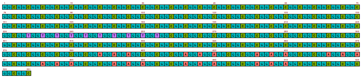
For all visualise_ functions, the render_device argument can be used to control the rendering method. It is fed directly to ggsave(device = ), so the ggsave documentation fully explains its use. The default ragg::agg_png works well and ensures consistent graphics (though not font) rendering across platforms/operating systems, so you should not need to change it.
4.2 Colour customisation
All of the colours used in the visualisation can be modified with the following arguments:
-
sequence_colours: A length-4 vector of the colours used for the boxes of A, C, G, and T respectively. -
sequence_text_colour: The colour used for the A, C, G, and T lettering inside the boxes. -
index_annotation_colour: The colour used for the index numbers above/below the boxes. -
background_colour: The colour used for the background. -
outline_colour: The colour used for the box outlines.
All colour-type arguments should accept colour, color, or col for the argument name.
For example, we can change all of the colours in an inadvisable way:
## Create image
visualise_single_sequence(
    sone_2019_f1_1_expanded_ggt_added,
    filename = paste0(output_location, "single_sequence_03.png"),
    return = FALSE,
    sequence_colors = c("black", "white", "#00FFFF", "#00FF00"),
    sequence_text_col = "magenta",
    index_annotation_colour = "yellow",
    background_color = "red",
    outline_colour = "orange"
)

## View image
view_image(paste0(display_location, "single_sequence_03.png"))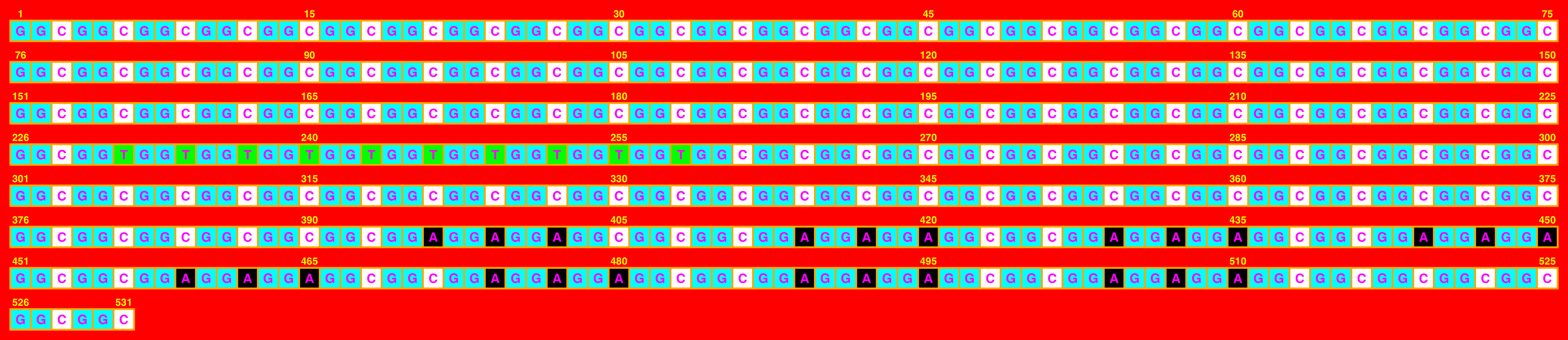
Included in ggDNAvis are a set of colour palettes for sequence colours that can often be helpful. The default is sequence_colour_palettes$ggplot_style, as seen in the first example above. The other palettes are $bright_pale, $bright_pale2, $bright_deep, $sanger, and $accessible:
The bright_pale palette works well with either white or black text, depending on how much the text is desired to “pop”:
## Create image
visualise_single_sequence(
    sone_2019_f1_1_expanded_ggt_added,
    filename = paste0(output_location, "single_sequence_04.png"),
    return = FALSE,
    sequence_colours = sequence_colour_palettes$bright_pale,
    sequence_text_colour = "white"
)

## View image
view_image(paste0(display_location, "single_sequence_04.png"))
## Create image
visualise_single_sequence(
    sone_2019_f1_1_expanded_ggt_added,
    filename = paste0(output_location, "single_sequence_05.png"),
    return = FALSE,
    sequence_colours = sequence_colour_palettes$bright_pale,
    sequence_text_colour = "black"
)

## View image
view_image(paste0(display_location, "single_sequence_05.png"))
bright_pale2 is the same but with a slightly lighter shade of green:
## Create image
visualise_single_sequence(
    sone_2019_f1_1_expanded_ggt_added,
    filename = paste0(output_location, "single_sequence_06.png"),
    return = FALSE,
    sequence_colours = sequence_colour_palettes$bright_pale2,
    sequence_text_colour = "black"
)

## View image
view_image(paste0(display_location, "single_sequence_06.png"))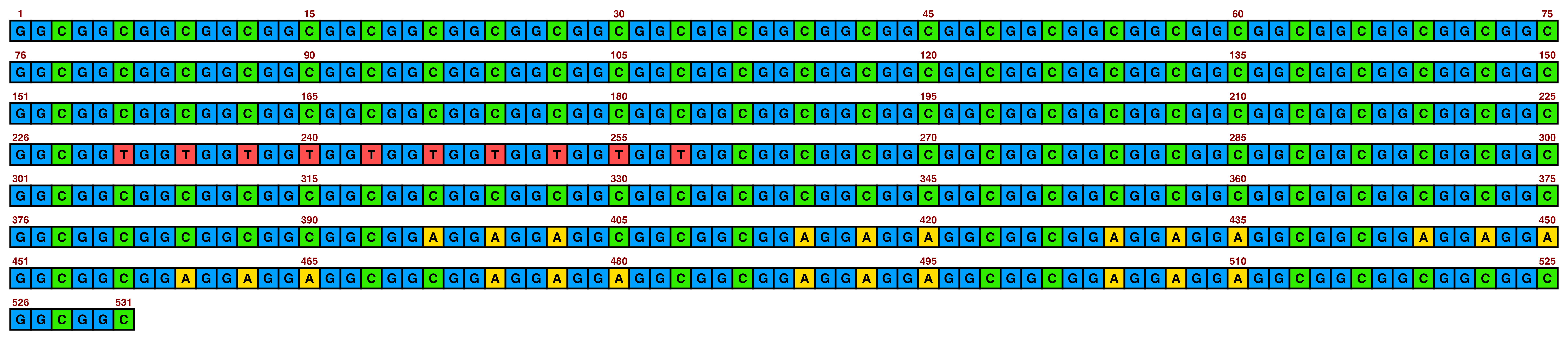
The bright_deep palette works best with white text:
## Create image
visualise_single_sequence(
    sone_2019_f1_1_expanded_ggt_added,
    filename = paste0(output_location, "single_sequence_07.png"),
    return = FALSE,
    sequence_colours = sequence_colour_palettes$bright_deep,
    sequence_text_colour = "white"
)

## View image
view_image(paste0(display_location, "single_sequence_07.png"))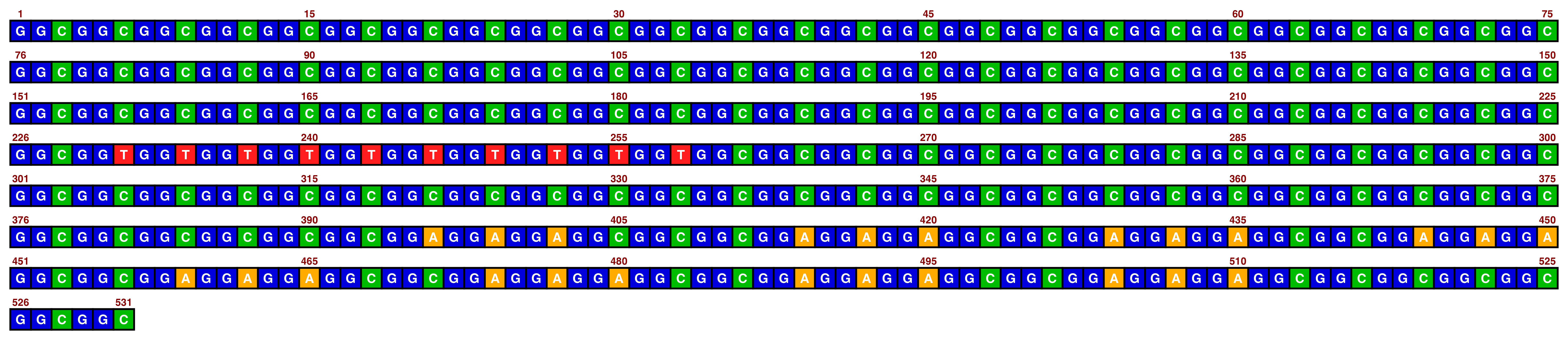
The sanger palette is inspired by old-school Sanger sequencing readouts and works best with white text:
## Create image
visualise_single_sequence(
    sone_2019_f1_1_expanded_ggt_added,
    filename = paste0(output_location, "single_sequence_08.png"),
    return = FALSE,
    sequence_colours = sequence_colour_palettes$sanger,
    sequence_text_colour = "white",
    outline_colour = "darkgrey"
)

## View image
view_image(paste0(display_location, "single_sequence_08.png"))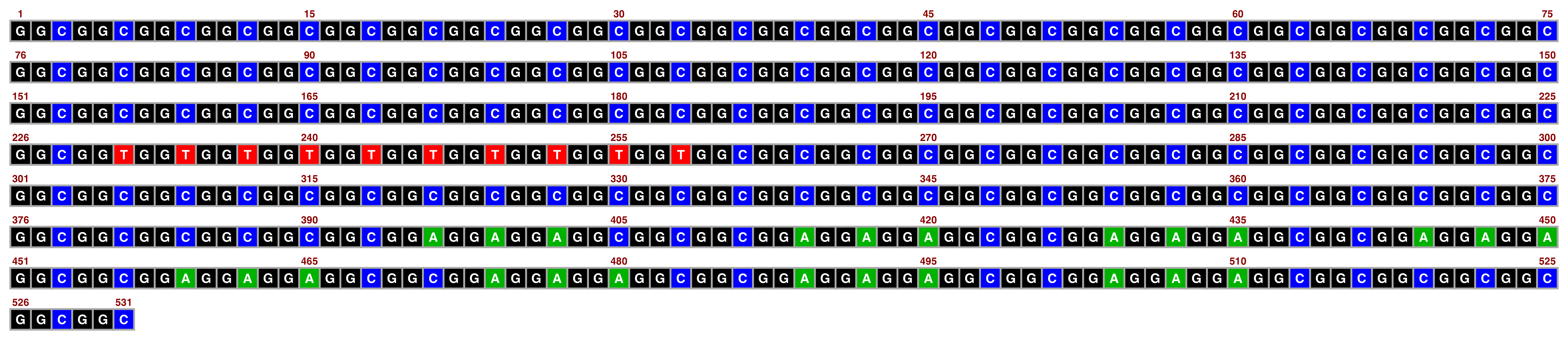
The accessible palette is light and dark each of blue and green, which is the only 4-category qualitative colourblind-safe palette recommended by colorbrewer2.org (Harrower & Brewer, 2003):
## Create image
visualise_single_sequence(
    sone_2019_f1_1_expanded_ggt_added,
    filename = paste0(output_location, "single_sequence_09.png"),
    return = FALSE,
    sequence_colours = sequence_colour_palettes$accessible,
    sequence_text_colour = "black"
)

## View image
view_image(paste0(display_location, "single_sequence_09.png"))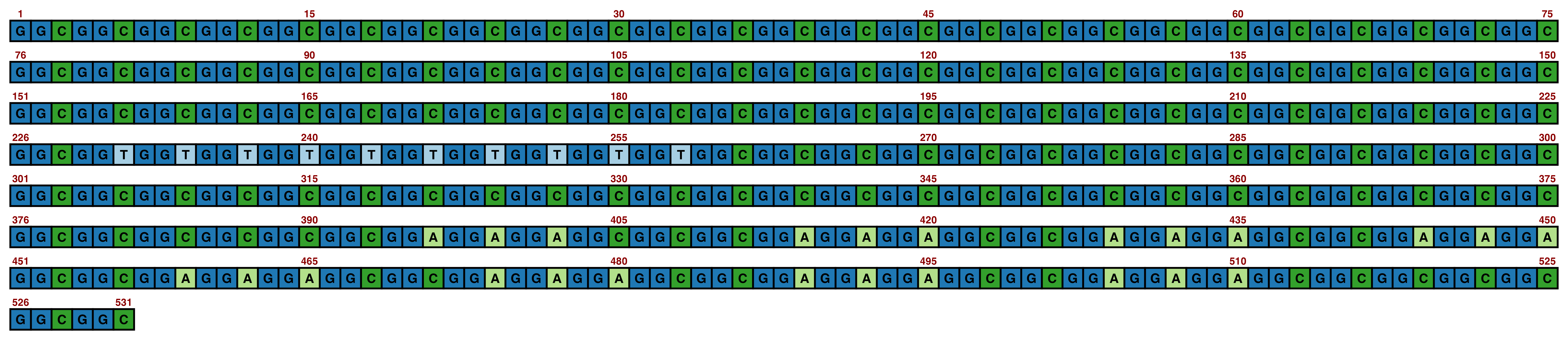
4.3 Layout customisation
Many aspects of the sequence layout are also customisable via arguments:
-
line_wrapping: The length/number of bases in each line. -
spacing: The number of blank lines in between each line of sequence. Must be an integer - this is a fundamental consequence of how the images are rasterised and the whole visualisation logic would need to be re-implemented to allow non-integer spacing values. -
margin: The margin around the image in terms of the size of base boxes (e.g. the default value of0.5adds a margin half the size of the base boxes, which is 50 px with the defaultpixels_per_base = 100). Note that if index annotations are on, there is a minimum margin of 1 above (if annotations are above) of below (if annotations are below) to allow space to render the annotations, so if margin is set to less than this then it will be increased to 1 in the relevant direction. Also note that if the margin is very narrow it can clip the box outlines, as they are rendered centred on the actual edge of the boxes (i.e. they “spill over” a little to each side if outline linewidth is non-zero), so placing the margin exactly at the box edges will cut half the outlines. -
sequence_text_size: The size of the text inside the boxes. Can be set to 0 to disable text inside boxes. Defaults to 16. -
index_annotation_size: The size of the index numbers above/below the boxes. Can be set to0to disable index annotations. Defaults to12.5. -
index_annotation_interval: The frequency at which index numbers should be listed. Can be set to0to disable index annotations. Defaults to15. -
index_annotations_above: Boolean specifying whether index annotations should be drawn above or below each line of sequence. Defaults toTRUE(above). -
index_annotation_vertical_position: How far annotation numbers should be rendered above (ifindex_annotations_above = TRUE) or below (ifindex_annotations_above = FALSE) each base. Defaults to1/3, not recommended to change generally. If spacing is much larger than1, setting this to a slightly higher value might be appropriate. -
index_annotation_always_first_base: Boolean specifying whether the first base should always be annotated even if it would not usually be (i.e.index_annotation_interval > 1). Defaults toTRUE. -
index_annotation_always_last_base: Boolean specifying whether the last base should always be annotated even if it would not usually be (i.e.line_length %% index_annotation_interval != 0). Defaults toTRUE. -
outline_linewidth: The thickness of the box outlines. Can be set to0to disable box outlines. Defaults to3. -
outline_join: Changes how the corners of the box outlines are handled. Must be one of"mitre","bevel", or"round". Defaults to"mitre". It is unlikely that you would ever need to change this.
A sensible example of how these might be changed is as follows:
## Create image
visualise_single_sequence(
    sone_2019_f1_1_expanded_ggt_added,
    filename = paste0(output_location, "single_sequence_10.png"),
    return = FALSE,
    sequence_colours = sequence_colour_palettes$ggplot_style,
    margin = 2,
    spacing = 2,
    line_wrapping = 60,
    index_annotation_interval = 20,
    index_annotations_above = FALSE,
    index_annotation_vertical_position = 1/2,
    index_annotation_always_first_base = FALSE,
    index_annotation_always_last_base = FALSE,
    outline_linewidth = 0
)

## View image
view_image(paste0(display_location, "single_sequence_10.png"))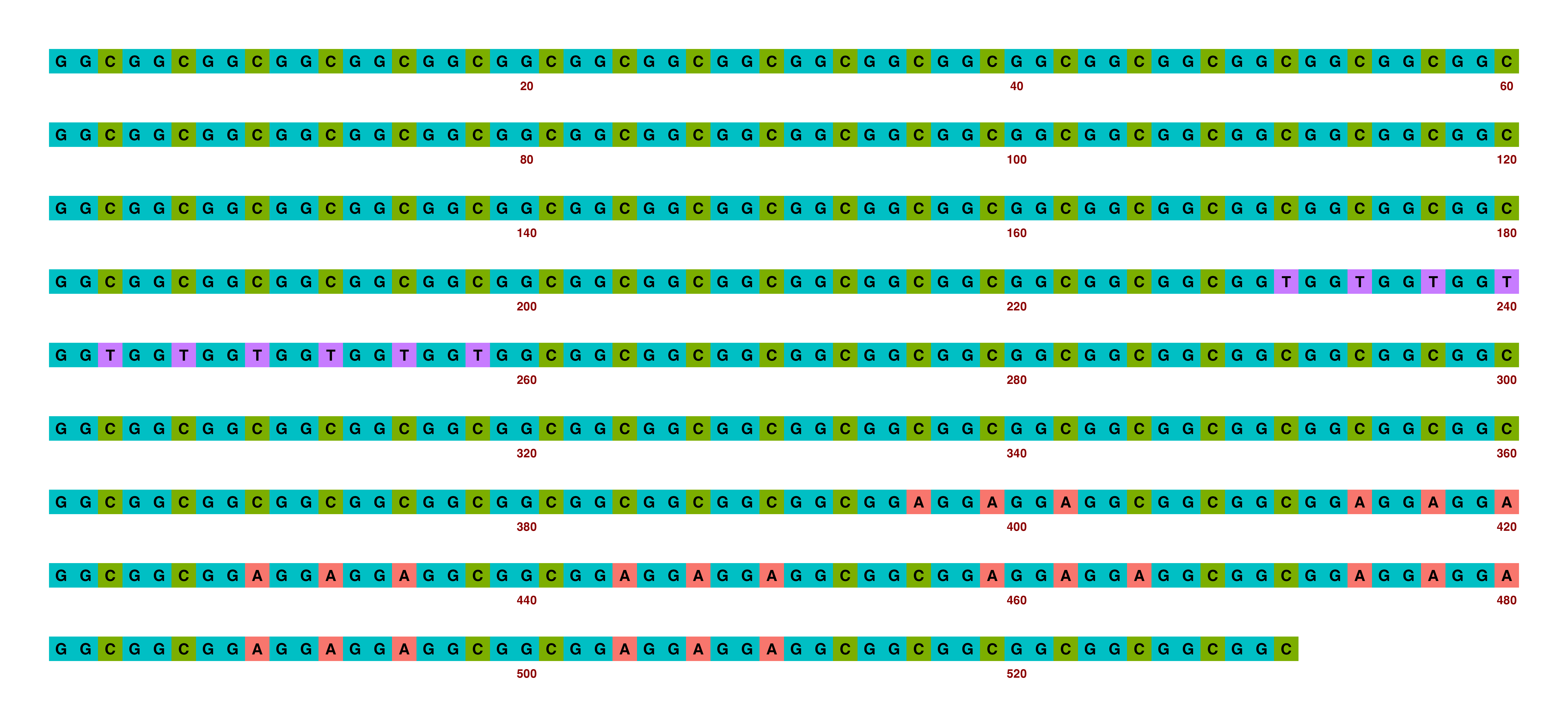
Setting spacing, margin, sequence text size, and index annotation interval all to 0 produces a no-frills visualisation of the sequence only. If doing so, pixels_per_base can be set low as there is no text that would be rendered poorly at low resolutions:
## Create image
visualise_single_sequence(
    sone_2019_f1_1_expanded_ggt_added,
    filename = paste0(output_location, "single_sequence_11.png"),
    return = FALSE,
    sequence_colours = sequence_colour_palettes$bright_pale,
    margin = 0,
    spacing = 0,
    line_wrapping = 45,
    sequence_text_size = 0,
    index_annotation_interval = 0,
    pixels_per_base = 20,
    outline_linewidth = 5
)
## Warning: Disabling index annotations via index_annotation_interval = 0 or index_annotation_size = 0 overrides the index_annotation_always_first_base setting.
## If you want the first base in each line to be annotated but no other bases, set index_annotation_interval greater than line_wrapping.
## Warning: Disabling index annotations via index_annotation_interval = 0 or index_annotation_size = 0 overrides the index_annotation_always_last_base setting.
## If you want the last base in each line to be annotated but no other bases, set index_annotation_interval greater than line_wrapping.
## Warning: If margin is small and outlines are on (outline_linewidth > 0), outlines may be cut off at the edges of the plot. Check if this is happening and consider using a bigger margin.
## Current margin: 0
## View image
view_image(paste0(display_location, "single_sequence_11.png"))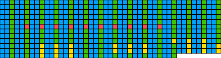 This produced a warning message as setting the margin to 0 clipped off the outlines of the outermost boxes. Either a slightly larger margin can be used:
## Create image
visualise_single_sequence(
    sone_2019_f1_1_expanded_ggt_added,
    filename = paste0(output_location, "single_sequence_12.png"),
    return = FALSE,
    sequence_colours = sequence_colour_palettes$bright_pale,
    margin = 0.3,
    spacing = 0,
    line_wrapping = 45,
    sequence_text_size = 0,
    index_annotation_interval = 0,
    pixels_per_base = 20,
    outline_linewidth = 3
)
## Warning: Disabling index annotations via index_annotation_interval = 0 or index_annotation_size = 0 overrides the index_annotation_always_first_base setting.
## If you want the first base in each line to be annotated but no other bases, set index_annotation_interval greater than line_wrapping.
## Warning: Disabling index annotations via index_annotation_interval = 0 or index_annotation_size = 0 overrides the index_annotation_always_last_base setting.
## If you want the last base in each line to be annotated but no other bases, set index_annotation_interval greater than line_wrapping.
## View image
view_image(paste0(display_location, "single_sequence_12.png"))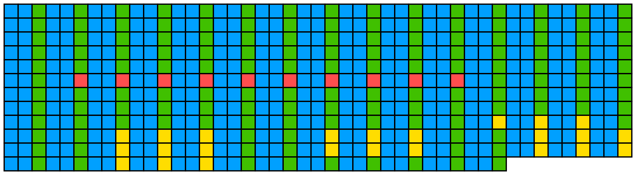
Or the outlines can be turned off:
## Create image
visualise_single_sequence(
sone_2019_f1_1_expanded_ggt_added,
filename = paste0(output_location, "single_sequence_13.png"),
return = FALSE,
sequence_colours = sequence_colour_palettes$bright_pale,
margin = 0,
spacing = 0,
line_wrapping = 45,
sequence_text_size = 0,
index_annotation_interval = 0,
pixels_per_base = 20,
outline_linewidth = 0
)## Warning: Disabling index annotations via index_annotation_interval = 0 or index_annotation_size = 0 overrides the index_annotation_always_first_base setting.
## If you want the first base in each line to be annotated but no other bases, set index_annotation_interval greater than line_wrapping.
## Warning: Disabling index annotations via index_annotation_interval = 0 or index_annotation_size = 0 overrides the index_annotation_always_last_base setting.
## If you want the last base in each line to be annotated but no other bases, set index_annotation_interval greater than line_wrapping.
## ℹ Automatically using geom_raster (much faster than geom_tile) as no sequence text, index annotations, or outlines are present.
## View image
view_image(paste0(display_location, "single_sequence_13.png"))
When changing line wrapping and annotation interval, divisibility is important. It is generally recommended to make the line wrapping length a multiple of the motif length when visualising repeats (e.g. a multiple of 3 for a trinucleotide repeat), and to make the index annotation interval a factor of the line wrapping length. If the annotation interval is not a factor of the line length, then there will be uneven gaps between annotations as the interval is counted from the start of each line.
Here is an example where these guidelines are not followed:
## Create image
visualise_single_sequence(
sone_2019_f1_1_expanded_ggt_added,
filename = paste0(output_location, "single_sequence_14.png"),
return = FALSE,
sequence_colours = sequence_colour_palettes$bright_deep,
sequence_text_colour = "white",
line_wrapping = 65,
index_annotation_interval = 15
)
## View image
view_image(paste0(display_location, "single_sequence_14.png"))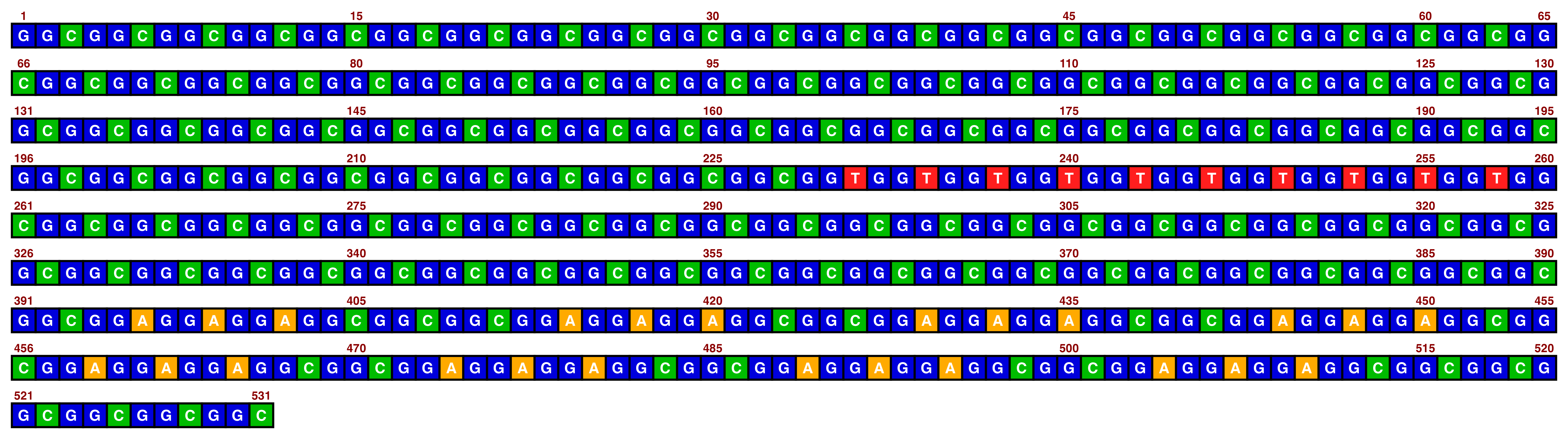
When setting spacing to 0, it is highly recommended to disable index annotations via index_annotation_interval = 0, otherwise there is nowhere for them to render:
## Create image
visualise_single_sequence(
sone_2019_f1_1_expanded_ggt_added,
filename = paste0(output_location, "single_sequence_15.png"),
return = FALSE,
sequence_colours = sequence_colour_palettes$sanger,
sequence_text_colour = "white",
index_annotation_colour = "magenta",
spacing = 0,
outline_colour = "magenta"
)## Warning: Using spacing = 0 without disabling index annotation is not recommended.
## It is likely to draw the annotations overlapping the sequence.
## Recommended to set index_annotation_interval = 0 to disable index annotations.
## View image
view_image(paste0(display_location, "single_sequence_15.png"))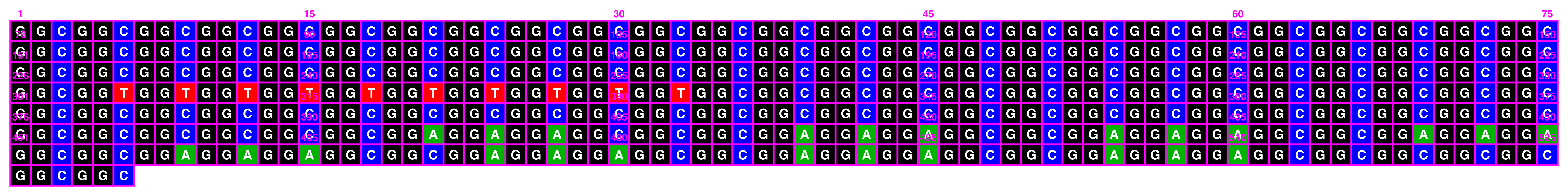
4.4 Performance
4.4.1 Performance monitoring
The four major visualise functions in ggDNAvis can track the time taken for each step of the visualisation processing. When the monitor_performance argument is set to TRUE, the date and timestamp will be printed along with the function name (obtained via Sys.time()). Then at the start of each processing step, the time since the start of the previous step (i.e. the time that the previous step took) will be printed along with total time since the start of the function.
For example:
## Create image
visualise_single_sequence(
sone_2019_f1_1_expanded_ggt_added,
filename = paste0(output_location, "single_sequence_16.png"),
return = FALSE,
monitor_performance = TRUE
)## ℹ Verbose monitoring enabled
## ℹ (2026-06-23 15:29:21) visualise_single_sequence start
## ℹ (0.003 secs elapsed; 0.003 secs total) resolving aliases
## ℹ (0.001 secs elapsed; 0.004 secs total) validating arguments
## ℹ (0.001 secs elapsed; 0.004 secs total) splitting input seq to sequence vector
## ℹ (0.002 secs elapsed; 0.007 secs total) rasterising image data
## ℹ (0.002 secs elapsed; 0.009 secs total) choosing rendering method
## ℹ (0.001 secs elapsed; 0.009 secs total) calculating tile sizes
## ℹ (0.001 secs elapsed; 0.010 secs total) creating basic plot via geom_tile
## ℹ (0.004 secs elapsed; 0.014 secs total) generating sequence text
## ℹ (0.001 secs elapsed; 0.014 secs total) adding sequence text
## ℹ (0.002 secs elapsed; 0.016 secs total) generating index annotations
## ℹ (0.001 secs elapsed; 0.017 secs total) adding index annotations
## ℹ (0.002 secs elapsed; 0.018 secs total) adding general plot themes
## ℹ (0.006 secs elapsed; 0.024 secs total) calculating margin
## ℹ (0.001 secs elapsed; 0.025 secs total) exporting image file
## ℹ (0.336 secs elapsed; 0.361 secs total) done
## View image
view_image(paste0(display_location, "single_sequence_16.png"))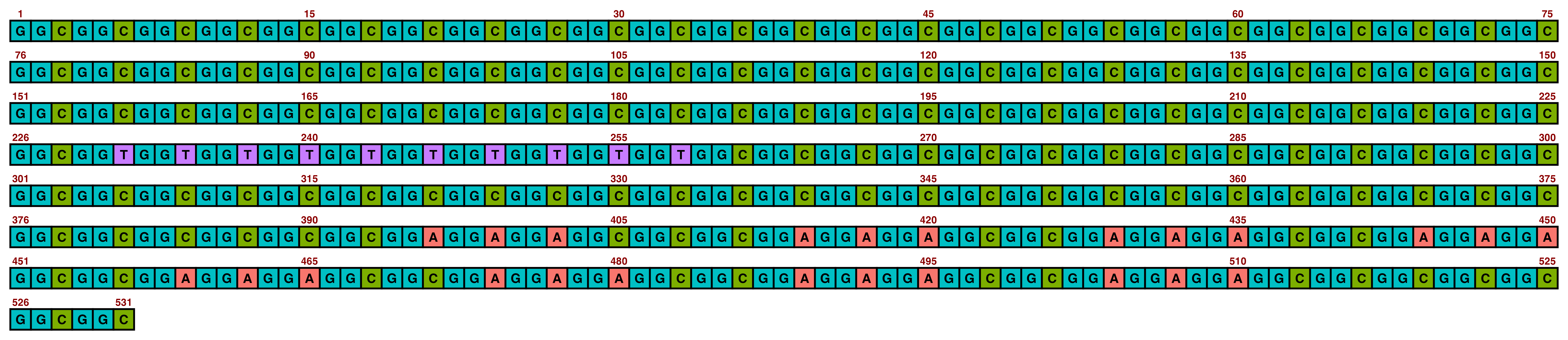
4.4.2 Raster versus tile rendering
Usually, visualisations in ggDNAvis are drawn via geom_tile(). This is highly customisable and allows box outlines, text superimposition, and index annotation. However, for very large datasets, rendering thousands or millions of tiles can become unusuably slow. A much faster alternative is geom_raster(), which does not allow for text/annotations/outlines but can draw much bigger images when needed.
geom_raster() is automatically used when it would not affect the output image (i.e. when sequence text, annotations, and outlines are already off), or can be forced by setting force_raster = TRUE. However, as forcing geom_raster() necessitates removal of text/annotations/outlines, this produces a warning unless they were all already turned off.
Furthermore, as geom_raster() only draws simple boxes, a message is produced if pixels_per_base is greater than 20, as there is not really any benefit and it increases the file size of the image.
An example where visualise_single_sequence() automatically switches to geom_raster() and produces a warning for excessive resolution is as follows:
## Create image
visualise_single_sequence(
sone_2019_f1_1_expanded_ggt_added,
filename = paste0(output_location, "single_sequence_17.png"),
return = FALSE,
sequence_colours = sequence_colour_palettes$bright_deep,
outline_linewidth = 0,
index_annotation_size = 0,
sequence_text_size = 0,
monitor_performance = TRUE
)## ℹ Verbose monitoring enabled
## ℹ (2026-06-23 15:29:21) visualise_single_sequence start
## ℹ (0.001 secs elapsed; 0.001 secs total) resolving aliases
## ℹ (0.001 secs elapsed; 0.002 secs total) validating arguments
## ℹ Automatically setting index_annotation_interval to 0 as index_annotation_size is 0
## Warning: Disabling index annotations via index_annotation_interval = 0 or index_annotation_size = 0 overrides the index_annotation_always_first_base setting.
## If you want the first base in each line to be annotated but no other bases, set index_annotation_interval greater than line_wrapping.

## Warning: Disabling index annotations via index_annotation_interval = 0 or index_annotation_size = 0 overrides the index_annotation_always_last_base setting.
## If you want the last base in each line to be annotated but no other bases, set index_annotation_interval greater than line_wrapping.
## ℹ (0.002 secs elapsed; 0.004 secs total) splitting input seq to sequence vector
## ℹ (0.001 secs elapsed; 0.004 secs total) rasterising image data
## ℹ (0.002 secs elapsed; 0.006 secs total) choosing rendering method
## ℹ Automatically using geom_raster (much faster than geom_tile) as no sequence text, index annotations, or outlines are present.
## Warning: When using geom_raster, it is recommended to use a smaller pixels_per_base e.g. 10, as there is no text/outlines that would benefit from higher resolution.
## Current value: 100
## ℹ (0.002 secs elapsed; 0.008 secs total) creating basic plot via geom_raster
## ℹ (0.003 secs elapsed; 0.011 secs total) adding general plot themes
## ℹ (0.007 secs elapsed; 0.018 secs total) calculating margin
## ℹ (0.001 secs elapsed; 0.019 secs total) exporting image file
## ℹ (0.371 secs elapsed; 0.390 secs total) done
## View image
view_image(paste0(display_location, "single_sequence_17.png"))
An example of forcing rasterisation when there would otherwise be sequence text, index annotations, and outlines (thus producing a warning) is as follows:
## Create image
visualise_single_sequence(
    sone_2019_f1_1_expanded_ggt_added,
    filename = paste0(output_location, "single_sequence_18.png"),
    return = FALSE,
    sequence_colours = sequence_colour_palettes$bright_deep,
    outline_linewidth = 5,
    outline_colour = "black",
    index_annotation_interval = 3,
    index_annotation_size = 12.5,
    index_annotation_colour = "darkred",
    sequence_text_size = 16,
    sequence_text_colour = "white",
    force_raster = TRUE,
    pixels_per_base = 10,
    monitor_performance = TRUE
)
## ℹ Verbose monitoring enabled
## ℹ (2026-06-23 15:29:22) visualise_single_sequence start
## ℹ (0.002 secs elapsed; 0.002 secs total) resolving aliases
## ℹ (0.001 secs elapsed; 0.002 secs total) validating arguments
## ℹ (0.001 secs elapsed; 0.003 secs total) splitting input seq to sequence vector
## ℹ (0.001 secs elapsed; 0.003 secs total) rasterising image data
## ℹ (0.001 secs elapsed; 0.005 secs total) choosing rendering method
## Warning: Forcing geom_raster via force_raster = TRUE will remove all sequence
## text, index annotations (though any inserted blank lines/spacers will remain),
## and box outlines.
## ℹ (0.001 secs elapsed; 0.006 secs total) creating basic plot via geom_raster
## ℹ (0.002 secs elapsed; 0.008 secs total) adding general plot themes
## ℹ (0.006 secs elapsed; 0.014 secs total) calculating margin
## ℹ (0.001 secs elapsed; 0.015 secs total) exporting image file
## ℹ (0.096 secs elapsed; 0.111 secs total) done
## View image
view_image(paste0(display_location, "single_sequence_18.png"))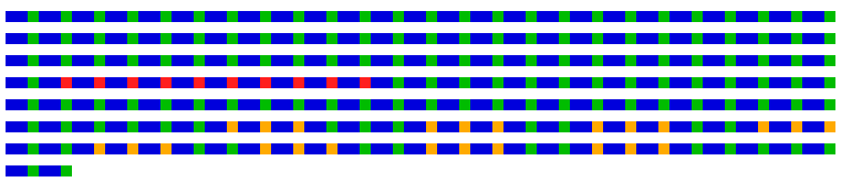
If sequence text, annotations, and outlines are all already off (i.e. sequence_text_size = 0, either index_annotation_size = 0 or index_annotation_interval = 0, and outline_linewidth = 0), then no warning is produced from force_raster (but it is redundant and doesn’t do anything):
## Create image
visualise_single_sequence(
    sone_2019_f1_1_expanded_ggt_added,
    filename = paste0(output_location, "single_sequence_19.png"),
    return = FALSE,
    sequence_colours = sequence_colour_palettes$bright_deep,
    outline_linewidth = 0,
    index_annotation_interval = 0,
    sequence_text_size = 0,
    pixels_per_base = 10,
    force_raster = TRUE,
    monitor_performance = TRUE
)
## ℹ Verbose monitoring enabled
## ℹ (2026-06-23 15:29:22) visualise_single_sequence start
## ℹ (0.002 secs elapsed; 0.002 secs total) resolving aliases
## ℹ (0.001 secs elapsed; 0.002 secs total) validating arguments
## Warning: Disabling index annotations via index_annotation_interval = 0 or index_annotation_size = 0 overrides the index_annotation_always_first_base setting.
## If you want the first base in each line to be annotated but no other bases, set index_annotation_interval greater than line_wrapping.
## Warning: Disabling index annotations via index_annotation_interval = 0 or index_annotation_size = 0 overrides the index_annotation_always_last_base setting.
## If you want the last base in each line to be annotated but no other bases, set index_annotation_interval greater than line_wrapping.
## ℹ (0.001 secs elapsed; 0.004 secs total) splitting input seq to sequence vector
## ℹ (0.001 secs elapsed; 0.004 secs total) rasterising image data
## ℹ (0.002 secs elapsed; 0.006 secs total) choosing rendering method
## ℹ Automatically using geom_raster (much faster than geom_tile) as no sequence text, index annotations, or outlines are present.
## ℹ (0.004 secs elapsed; 0.010 secs total) creating basic plot via geom_raster
## ℹ (0.003 secs elapsed; 0.013 secs total) adding general plot themes
## ℹ (0.007 secs elapsed; 0.020 secs total) calculating margin
## ℹ (0.001 secs elapsed; 0.021 secs total) exporting image file
## ℹ (0.099 secs elapsed; 0.120 secs total) done
## View image
view_image(paste0(display_location, "single_sequence_19.png"))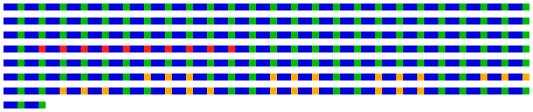
5 Visualising many DNA/RNA sequences
5.1 Basic visualisation
ggDNAvis can be used to visualise multiple DNA sequences via visualise_many_sequences(). This function takes a vector of sequences as its primary input, which do not all have to be the same length and can be blank for spacing lines. This can be constructed manually e.g. c("GGCGGCGGC", "", "TTATTA"), but is more easily produced by extract_and_sort_sequences().
Here is an example of how that could be accomplished with the example_many_sequences data, with a reminder of how to load sequence/quality data from FASTQ and merge with metadata (as fully explained in the reading standard FASTQ section):
## Reminder of how to load data from file
fastq_data <- read_fastq(
    system.file("extdata/example_many_sequences_raw.fastq", package = "ggDNAvis"),
    calculate_length = TRUE
)
metadata   <- read.csv(system.file("extdata/example_many_sequences_metadata.csv", package = "ggDNAvis"))
merged_fastq_data <- merge_fastq_with_metadata(fastq_data, metadata)

## Subset and change colnames to make it match example_many_sequences
merged_fastq_data <- merged_fastq_data[, c("family", "individual", "read", "forward_sequence", "sequence_length", "forward_quality")]
colnames(merged_fastq_data)[c(4,6)] <- c("sequence", "quality")

## Prove equivalance to example_many_sequences
identical(merged_fastq_data, example_many_sequences[, 1:6])
## Look at first 4 rows of the data as a reminder
print_table(head(merged_fastq_data, 4))| family | individual | read | sequence | sequence_length | quality |
|---|---|---|---|---|---|
Family 1 |
F1-1 |
F1-1a |
GGCGGCGGCGGCGGCGGCGGCGGCGGCGGAGGAGGCGGCGGCGGAGGAGGCGGCGGCGGAGGAGGCGGCGGCGGAGGAGGCGGCGGCGGAGGAGGCGGCGGA |
102 |
)8@!9:/0/,0+-6?40,-I601:.';+5,@0.0%)!(20C*,2++*(00#/*+3;E-E)<I5.5G*CB8501;I3'.8233'3><:13)48F?09*>?I90 |
Family 1 |
F1-1 |
F1-1b |
GGCGGCGGCGGCGGCGGCGGCGGCGGCGGCGGCGGAGGAGGCGGCGGCGGAGGAGGCGGCGGA |
63 |
60-7,7943/*=5=)7<53-I=G6/&/7?8)<$12">/2C;4:9F8:816E,6C3*,1-2139 |
Family 1 |
F1-1 |
F1-1c |
GGCGGCGGCGGCGGCGGCGGCGGCGGCGGAGGAGGCGGCGGCGGAGGAGGCGGCGGCGGAGGAGGCGGCGGCGGAGGAGGCGGCGGA |
87 |
;F42DF52#C-*I75!4?9>IA0<30!-:I:;+7!:<7<8=G@5*91D%193/2;><IA8.I<.722,68*!25;69*<<8C9889@ |
Family 1 |
F1-1 |
F1-1d |
GGCGGCGGCGGCGGCGGCGGCGGCGGCGGCGGCGGCGGAGGAGGCGGCGGCGGAGGAGGCGGCGGCGGAGGAGGCGGCGGA |
81 |
:<*1D)89?27#8.3)9<2G<>I.=?58+:.=-8-3%6?7#/FG)198/+3?5/0E1=D9150A4D//650%5.@+@/8>0 |
## Extract sequences to a character vector
sequences_for_visualisation <- extract_and_sort_sequences(merged_fastq_data)

## View the character vector
sequences_for_visualisation
## [1] "GGCGGCGGCGGCGGCGGCGGCGGCGGCGGAGGAGGCGGCGGCGGAGGAGGCGGCGGCGGAGGAGGCGGCGGCGGAGGAGGCGGCGGCGGAGGAGGCGGCGGA"
## [2] "GGCGGCGGCGGCGGCGGCGGAGGAGGCGGCGGCGGAGGAGGCGGCGGCGGAGGAGGCGGCGGCGGAGGAGGCGGCGGCGGAGGAGGCGGCGGA"
## [3] "GGCGGCGGCGGCGGCGGCGGCGGCGGCGGAGGAGGCGGCGGCGGAGGAGGCGGCGGCGGAGGAGGCGGCGGCGGAGGAGGCGGCGGA"
## [4] "GGCGGCGGCGGCGGCGGCGGCGGCGGCGGCGGCGGCGGAGGAGGCGGCGGCGGAGGAGGCGGCGGCGGAGGAGGCGGCGGA"
## [5] "GGCGGCGGCGGCGGCGGCGGCGGCGGCGGCGGCGGAGGAGGCGGCGGCGGAGGAGGCGGCGGA"
## [6] ""
## [7] ""
## [8] "GGCGGCGGCGGCGGCGGCGGCGGCGGCGGCGGCGGCGGAGGAGGAGGCGGCGGAGGAGGAGGCGGCGGA"
## [9] "GGCGGCGGCGGCGGCGGCGGCGGCGGCGGCGGAGGAGGAGGCGGCGGAGGAGGAGGCGGCGGA"
## [10] ""
## [11] ""
## [12] "GGCGGCGGCGGCGGCGGCGGCGGCGGCGGAGGAGGCGGCGGCGGAGGAGGCGGCGGCGGAGGAGGCGGCGGCGGAGGAGGCGGCGGA"
## [13] "GGCGGCGGCGGCGGCGGCGGCGGCGGCGGAGGAGGCGGCGGCGGAGGAGGCGGCGGCGGAGGAGGCGGCGGAGGAGGCGGCGGA"
## [14] "GGCGGCGGCGGCGGCGGCGGCGGCGGCGGCGGCGGCGGCGGCGGCGGAGGAGGCGGCGGCGGAGGAGGCGGCGGCGGCGGA"
## [15] ""
## [16] ""
## [17] ""
## [18] ""
## [19] ""
## [20] ""
## [21] ""
## [22] ""
## [23] "GGCGGCGGCGGCGGCGGCGGCGGCGGCGGCGGCGGCGGCGGCGGCGGCGGCGGCGGCGGCGGCGGCGGCGGCGGCGGCGGAGGAGGCGGCGGA"
## [24] ""
## [25] ""
## [26] "GGCGGCGGCGGCGGCGGCGGCGGCGGCGGCGGCGGCGGCGGCGGCGGCGGCGGCGGCGGCGGCGGCGGCGGCGGCGGAGGAGGCGGCGGA"
## [27] "GGCGGCGGCGGCGGCGGCGGCGGCGGCGGCGGCGGCGGCGGCGGCGGCGGCGGCGGCGGCGGCGGCGGCGGCGGAGGAGGCGGCGGA"
## [28] "GGCGGCGGCGGCGGCGGCGGCGGCGGCGGCGGCGGCGGCGGCGGCGGCGGCGGCGGCGGCGGCGGCGGCGGAGGAGGCGGCGGA"
## [29] ""
## [30] ""
## [31] ""
## [32] ""
## [33] ""
## [34] ""
## [35] ""
## [36] ""
## [37] "GGCGGCGGCGGTGGTGGCGGCGGTGGTGGCGGCGGTGGTGGCGGCGGTGGTGGCGGCGGTGGTGGCGGCGGTGGTGGCGGCGGTGGTGGCGGCGGA"
## [38] "GGCGGCGGCGGCGGCGGCGGCGGTGGTGGCGGCGGTGGTGGCGGCGGTGGTGGCGGCGGTGGTGGCGGCGGTGGTGGCGGCGGTGGTGGCGGCGGA"
## [39] ""
## [40] ""
## [41] "GGCGGCGGCGGCGGCGGCGGTGGTGGCGGCGGTGGTGGCGGCGGTGGTGGCGGCGGTGGTGGCGGCGGTGGTGGCGGCGGTGGTGGCGGCGGA"
## [42] "GGCGGCGGCGGCGGCGGCGGTGGTGGCGGCGGTGGTGGCGGCGGTGGTGGCGGCGGTGGTGGCGGCGGTGGTGGCGGCGGTGGTGGCGGA"
## [43] "GGCGGCGGCGGCGGCGGCGGCGGCGGCGGCGGAGGAGGCGGCGGAGGAGGCGGCGGAGGAGGCGGCGGAGGAGGCGGCGGCGGCGGA"
## [44] ""
## [45] ""
## [46] "GGCGGCGGCGGCGGCGGCGGCGGTGGTGGCGGCGGTGGTGGCGGCGGTGGTGGCGGCGGTGGTGGCGGCGGTGGTGGCGGCGGTGGTGGCGGCGGA"
## [47] ""
## [48] ""
## [49] "GGCGGCGGCGGCGGCGGCGGCGGCGGCGGCGGCGGTGGTGGCGGCGGTGGTGGCGGCGGTGGTGGCGGCGGTGGTGGCGGCGGTGGTGGCGGCGGA"
## [50] "GGCGGCGGCGGCGGCGGCGGCGGCGGAGGAGGCGGCGGAGGAGGCGGCGGAGGAGGCGGCGGAGGAGGCGGCGGAGGAGGCGGCGGCGGA"
## [51] "GGCGGCGGCGGCGGCGGCGGCGGCGGCGGCGGCGGCGGTGGTGGCGGCGGTGGTGGCGGCGGTGGTGGCGGCGGCGGCGGA"
## Use the character vector to make the image
visualise_many_sequences(
sequences_for_visualisation,
filename = paste0(output_location, "many_sequences_01.png"),
return = FALSE
)
## View image
view_image(paste0(display_location, "many_sequences_01.png"))
5.2 Sequence arrangement customisation
The extract_and_sort_sequences() function is highly configurable to change the arrangement and spacing of the sequences.
It takes the following arguments:
-
sequence_dataframe: The data to be processed -
sequence_variable: The name of the column we are extracting. This doesn’t actually have to be a sequence, it could be any information that we want to convert into a sorted vector spaced out with empty strings. -
grouping_levels: How the data should be grouped. This is a named numerical vector stating which variables/columns should be used to group the data, and how many lines should be left between groups at each level. For example, the defaultc("family" = 8, "individual" = 2)means the top-level grouping is done by categories in the"family"column and there are 8 blank lines between each family, and the second-level grouping is done by the"individual"column and there are 2 blank lines between individuals within the same family. This is implemented recursively, so any number of grouping variables can be used (or this can be set toNAto turn off grouping entirely). -
sort_by: The name of the column used to sort sequences within the lowest-level groups. This is generally the sequence length (but doesn’t have to be). -
desc_sort: Whether the sequences should be sorted by thesort_byvariable descending (desc_sort = TRUE) or (desc_sort = FALSE).
The image above used all the default values, which are set up to work with the columns present in example_many_sequences and use the families-separated-by-8, individuals-separated-by-2 grouping and arranged sequences in descending length order.
Here is the same image but with the default arguments explicitly stated:
## Extract sequences to a character vector
## Remember that example_many_sequences is identical to the data
## read from FASTQ and metadata CSV in the previous code section
sequences_for_visualisation <- extract_and_sort_sequences(
example_many_sequences,
sequence_variable = "sequence",
grouping_levels = c("family" = 8,
"individual" = 2),
sort_by = "sequence_length",
desc_sort = TRUE
)
## We will not view the character vector in the interests of avoiding clutter.
## Use the character vector to make the image
visualise_many_sequences(
sequences_for_visualisation,
filename = paste0(output_location, "many_sequences_02.png"),
return = FALSE
)
## View image
view_image(paste0(display_location, "many_sequences_02.png"))
Here the top large cluster is Family 1, containing individuals F1-1, F1-2, and F-3. These individuals contain 5, 2, and 3 reads respectively, and are separated from each other by 2 blank lines. After Family 1, there is there 8 blank lines before Family 2. Family 2 contains F2-1 and F2-2 with 1 and 3 reads (individuals separated by 2 blank lines), then there are 8 blank lines before Family 3. Family 3 contains F3-1, F3-2, F3-3, and F3-4 with 2, 3, 1, and 3 reads.
If we wanted to group only by individual without showing the family structure, and present reads in ascending length order for each individual, we could do the following:
## Extract sequences to a character vector
sequences_for_visualisation <- extract_and_sort_sequences(
example_many_sequences,
sequence_variable = "sequence",
grouping_levels = c("individual" = 1),
sort_by = "sequence_length",
desc_sort = FALSE
)
## Use the character vector to make the image
visualise_many_sequences(
sequences_for_visualisation,
filename = paste0(output_location, "many_sequences_03.png"),
return = FALSE
)
## View image
view_image(paste0(display_location, "many_sequences_03.png"))
Now we have a group for each individual, with sequences in ascending length order per individual, and one blank line between individuals.
We could also turn off grouping entirely to just visualise all of the reads in length order, via grouping_levels = NA:
## Extract sequences to a character vector
sequences_for_visualisation <- extract_and_sort_sequences(
example_many_sequences,
sequence_variable = "sequence",
grouping_levels = NA,
sort_by = "sequence_length",
desc_sort = TRUE
)
## Use the character vector to make the image
visualise_many_sequences(
sequences_for_visualisation,
filename = paste0(output_location, "many_sequences_04.png"),
return = FALSE
)
## View image
view_image(paste0(display_location, "many_sequences_04.png"))
We can also turn off sorting entirely (keeping grouping off) with sort_by = NA to simply show all the reads in the order in which they appear in the dataframe:
NB: if sort_by = NA is used, then desc_sort does nothing so it doesn’t matter what it is set to.
## Extract sequences to a character vector
sequences_for_visualisation <- extract_and_sort_sequences(
example_many_sequences,
sequence_variable = "sequence",
grouping_levels = NA,
sort_by = NA
)
## Use the character vector to make the image
visualise_many_sequences(
sequences_for_visualisation,
filename = paste0(output_location, "many_sequences_05.png"),
return = FALSE
)
## View image
view_image(paste0(display_location, "many_sequences_05.png"))
It is also possible to keep grouping on while turning sorting off if desired:
## Extract sequences to a character vector
sequences_for_visualisation <- extract_and_sort_sequences(
example_many_sequences,
sequence_variable = "sequence",
grouping_levels = c("family" = 2,
"individual" = 1),
sort_by = NA
)
## Use the character vector to make the image
visualise_many_sequences(
sequences_for_visualisation,
filename = paste0(output_location, "many_sequences_06.png"),
return = FALSE
)
## View image
view_image(paste0(display_location, "many_sequences_06.png"))
The grouping spacers can be set to 0 to sort within groups without visually separating them (but negative values don’t work - they produce an error in rep() as the blank line can’t be repeated a negative number of times). Additionally, the order of the groups/levels within a grouping variable can be changed in standard R fashion with factor(x, levels = ...):
## Reorder families
example_many_sequences_reordered <- example_many_sequences
example_many_sequences_reordered$family_reordered <- factor(
example_many_sequences_reordered$family,
levels = c("Family 2",
"Family 3",
"Family 1")
)
## Extract sequences to a character vector
sequences_for_visualisation <- extract_and_sort_sequences(
example_many_sequences_reordered,
sequence_variable = "sequence",
grouping_levels = c("family_reordered" = 0),
sort_by = "sequence_length"
)
## Use the character vector to make the image
visualise_many_sequences(
sequences_for_visualisation,
filename = paste0(output_location, "many_sequences_07.png"),
return = FALSE
)
## View image
view_image(paste0(display_location, "many_sequences_07.png"))
Finally, all the same grouping and sorting logic can be used to extract any other column as a character vector, though of course if it isn’t DNA sequence then the resulting vector is not valid input to visualise_many_sequences(). The column for extraction is specified by sequence_variable, and the column for sorting is sort_by. If the sort_by column is non-numeric then it will be sorted alphabetically, just like using sort() on a character vector.
## Extract qualities to character vector,
## sorted alphabetically by quality string
extracted_and_sorted_qualities <- extract_and_sort_sequences(
example_many_sequences,
sequence_variable = "quality",
grouping_levels = c("family" = 2),
sort_by = "quality",
desc_sort = FALSE
)
## View character vector
print(extracted_and_sorted_qualities, quote = F)## [1] )8@!9:/0/,0+-6?40,-I601:.';+5,@0.0%)!(20C*,2++*(00#/*+3;E-E)<I5.5G*CB8501;I3'.8233'3><:13)48F?09*>?I90
## [2] *46.5//3:37?24:(:0*#.))E)?:,/172=2!4">.*/;"8+5<;D6.I2=>:C3)108,<)GC161)!55E!.>86/
## [3] 60-7,7943/*=5=)7<53-I=G6/&/7?8)<$12">/2C;4:9F8:816E,6C3*,1-2139
## [4] 736/A@B121C269<2I,'5G66>46A6-9*&4*;4-E4C429?I+3@83(234E0%:43;!/3;2+956A0)(+'5G4=*3;1
## [5] :<*1D)89?27#8.3)9<2G<>I.=?58+:.=-8-3%6?7#/FG)198/+3?5/0E1=D9150A4D//650%5.@+@/8>0
## [6] ;4*2E3-48?@6A-!00!;-3%:H,4H>H530C(85I/&75-62.:2#!/D=A?8&7E!-@:=::5,)51,97D*04'2.!20@/;6)947<6
## [7] ;F42DF52#C-*I75!4?9>IA0<30!-:I:;+7!:<7<8=G@5*91D%193/2;><IA8.I<.722,68*!25;69*<<8C9889@
## [8] ?;.*26<C-8B,3#8/,-9!1++:94:/!A317=9>502=-+8;$=53@D*?/6:6&0D7-.@8,5;F,1?0D?$9'&665B8.604
## [9] E6(<)"-./EE<(5:47,(C818I9CC1=.&)4G6-7<(*"(,2C>8/5:0@@).A$97I!-<
## [10] F='I#*5I:<F?)<4G3&:95*-5?1,!:9BD4B5.-27577<2E9)2:189B.5/*#7;;'**.7;-!
## [11]
## [12]
## [13] 7?38,EC#3::=1)8&;<">3.9BE)1661!2)5-4.11B<3)?')-+,B4.<7)/:IE=5$.3:66G9216-C20,>(0848(1$-
## [14] ;1>:5417*<1.2H#260197.;7<(-3?0+=:)ID'I$6*128*!4.7-=5;+384F!=5>4!93+.6I7+H1-).H><68;7
## [15] =</-I354/,*>+<CA40*537/;<@I7/4%6192'5'>#4:&C,072+90:0+4;74"D5,38&<7A?00+1>G>#=?;,@<<1=64D=!1&
## [16] @86,/+6=8/;9=1)48E494IB3456/6.*=</B32+5469>8?@!1;*+81$>-99D7<@1$6B'?462?CE+=1+95=G?.6CA%>2
## [17]
## [18]
## [19] $<,5"7+!$';8<0794*@FI>34224!57+#1!F<+53$,?)-.A3;=1*71C02<.5:1)82!86$03/;%+1C3+D3;@9B-E#+/70;9<D'
## [20] .85$#;!1F$8E:B+;7CI6@11/'65<3,4G:8@GF1413:0)3CH1=44.%G=#2E67=?;9DF7358.;(I!74:1I4
## [21] /*2<C643?*8?@9)-.'5A!=3-=;6,.%H3-!10'I>&@?;96;+/+36;:C;B@/=:6,;61>?>!,>.97@.48B38(;7;1F464=-7;)7
## [22] /C<$>7/1(9%4:6>6I,D%*,&D?C/6@@;7)83.E.7:@9I906<!4536!850!164/8,<=?=15A;8B/5B364A66.1%9=(9876E8C:
## [23] 0/2>@/6+-/(!=9-?G!AA70*,/!/?-E46:,-1G94*491,,38?(-!6<8A;/C9;,3)4C06=%',86A)1!E@/24G59<<
## [24] 5@<733';9+3BB)=69,3!.2B*86'8E>@3?!(36:<002/4>:1.43A!+;<.3G*G8?0*991,B(C/"I9*1-86)8.;;5-0+=
## [25] 9>124!752+@06I/.72097*';-+A60=B?+/8'15477>4-435D;G@G'./21:(0/1/A=7'I>A"3=9;;12,@"2=3D=,458
## [26] :0I4099<,4E01;/@96%2I2<,%<C&=81F+4<*@4A5.('4!%I3CE657<=!5;37>4D:%3;7'"4<.9;?;7%0>:,84B512,B7/
## [27] ?2-#-2"1:(5(4>!I)>I,.?-+EG3IH4-.C:;570@2I;?D5#/;A7=>?<3?080::459*?8:3"<2;I)C1400)6:3%19./);.I?35This extracted the quality column, with families separated by 2 blank strings, and sorted alphabetically by quality string within each family.
5.3 Index annotation customisation
As of ggDNAvis v1.0.0, visualise_many_sequences() (and visualise_methylation()) support index annotation. This is implemented differently to visualise_single_sequence() because each line represents a different sequence/read, so it would not make sense to maintain a single base count. Instead, base indices are counted along each line and reset for each new line. To reduce redundancy, it is user-configurable which lines are annotated.
The full set of arguments controlling index annotations are:
-
index_annotation_lines: This is a key argument to change. Controls which lines should have their indices annotated. Defaults to1i.e. only the first line will be annotated. Can be set to1:length(sequences_vector)to annotate all lines, or to a custom integer vector to annotate specific lines. With the default argument values ofextract_and_sort_sequences(),c(1, 23, 37)annotates the first sequence from each family, which I personally find a useful setting. It may take some trial and error to find the ideal setting of this for each ordering/dataset. Can be set to0,FALSE,NA,NULL, ornumeric(0)to disable index annotations. -
index_annotation_full_line: Whether the annotations should always continue to the end of the longest sequence (TRUE, default) or whether they should end once the sequence along each annotated line ends (FALSE). -
index_annotation_colour: The colour used for the index numbers above/below the boxes. Defaults to dark red. -
index_annotation_size: The size of the index numbers above/below the boxes. Can be set to0to disable index annotations. Defaults to12.5. -
index_annotation_interval: The frequency at which index numbers should be listed. Defaults to15. Note that unlikevisualise_single_sequence(), the count resets each line invisualise_many_sequences()andvisualise_methylation()because each line is assumed to be a different sequence. -
index_annotations_above: Boolean specifying whether index annotations should be drawn above or below each line of sequence. Defaults toTRUE(above). -
index_annotation_always_first_base: Boolean specifying whether the first base should always be annotated even if it would not usually be (i.e.index_annotation_interval > 1). Defaults toTRUE. Note that this only applies to lines where annotations would be drawn, so not if they are excluded byindex_annotation_linesor disabled viaindex_annotation_interval = 0orindex_annotation_size = 0. If the goal is to annotate the first base and no others in each line, turn this on but setindex_annotation_intervalto a value greater than the maximum sequence length. -
index_annotation_always_last_base: Boolean specifying whether the last base should always be annotated even if it would not usually be (i.e.line_length %% index_annotation_interval != 0). Defaults toTRUE. -
index_annotation_vertical_position: How far annotation numbers should be rendered above (ifindex_annotations_above = TRUE) or below (ifindex_annotations_above = FALSE) each base. Defaults to1/3, not recommended to change generally.
We will work through these arguments step by step to fully explain how they work.
By default, annotations are drawn above the first line:
## Extract sequences to a character vector, using all default settings
sequences_for_visualisation <- extract_and_sort_sequences(example_many_sequences)
## Use the character vector to make the image
## index_annotation_lines = c(1) is the default value
visualise_many_sequences(
sequences_for_visualisation,
filename = paste0(output_location, "many_sequences_08.png"),
return = FALSE,
sequence_colours = sequence_colour_palettes$bright_pale2,
index_annotation_lines = c(1)
)
## View image
view_image(paste0(display_location, "many_sequences_08.png"))
However, any numerical vector can be used as index_annotation_lines to specify which lines should be annotated. For each selected line, an additional blank/spacer line will be inserted above (if index_annotations_above = TRUE) or below (if index_annotations_below = FALSE), and index annotations will be drawn in the new space.
(Note: if index_annotation_vertical_position is more than 1, more than 1 additional blank line will be inserted, according to ceiling(index_annotation_vertical_position)).
Annotating above each line would look as follows:
visualise_many_sequences(
sequences_for_visualisation,
filename = paste0(output_location, "many_sequences_09.png"),
return = FALSE,
sequence_colours = sequence_colour_palettes$bright_pale2,
index_annotation_lines = c(1:51)
)
## View image
view_image(paste0(display_location, "many_sequences_09.png"))
To annotate below the final line of each family, we can look at the sequences vector:
sequences_for_visualisation## [1] "GGCGGCGGCGGCGGCGGCGGCGGCGGCGGAGGAGGCGGCGGCGGAGGAGGCGGCGGCGGAGGAGGCGGCGGCGGAGGAGGCGGCGGCGGAGGAGGCGGCGGA"
## [2] "GGCGGCGGCGGCGGCGGCGGAGGAGGCGGCGGCGGAGGAGGCGGCGGCGGAGGAGGCGGCGGCGGAGGAGGCGGCGGCGGAGGAGGCGGCGGA"
## [3] "GGCGGCGGCGGCGGCGGCGGCGGCGGCGGAGGAGGCGGCGGCGGAGGAGGCGGCGGCGGAGGAGGCGGCGGCGGAGGAGGCGGCGGA"
## [4] "GGCGGCGGCGGCGGCGGCGGCGGCGGCGGCGGCGGCGGAGGAGGCGGCGGCGGAGGAGGCGGCGGCGGAGGAGGCGGCGGA"
## [5] "GGCGGCGGCGGCGGCGGCGGCGGCGGCGGCGGCGGAGGAGGCGGCGGCGGAGGAGGCGGCGGA"
## [6] ""
## [7] ""
## [8] "GGCGGCGGCGGCGGCGGCGGCGGCGGCGGCGGCGGCGGAGGAGGAGGCGGCGGAGGAGGAGGCGGCGGA"
## [9] "GGCGGCGGCGGCGGCGGCGGCGGCGGCGGCGGAGGAGGAGGCGGCGGAGGAGGAGGCGGCGGA"
## [10] ""
## [11] ""
## [12] "GGCGGCGGCGGCGGCGGCGGCGGCGGCGGAGGAGGCGGCGGCGGAGGAGGCGGCGGCGGAGGAGGCGGCGGCGGAGGAGGCGGCGGA"
## [13] "GGCGGCGGCGGCGGCGGCGGCGGCGGCGGAGGAGGCGGCGGCGGAGGAGGCGGCGGCGGAGGAGGCGGCGGAGGAGGCGGCGGA"
## [14] "GGCGGCGGCGGCGGCGGCGGCGGCGGCGGCGGCGGCGGCGGCGGCGGAGGAGGCGGCGGCGGAGGAGGCGGCGGCGGCGGA"
## [15] ""
## [16] ""
## [17] ""
## [18] ""
## [19] ""
## [20] ""
## [21] ""
## [22] ""
## [23] "GGCGGCGGCGGCGGCGGCGGCGGCGGCGGCGGCGGCGGCGGCGGCGGCGGCGGCGGCGGCGGCGGCGGCGGCGGCGGCGGAGGAGGCGGCGGA"
## [24] ""
## [25] ""
## [26] "GGCGGCGGCGGCGGCGGCGGCGGCGGCGGCGGCGGCGGCGGCGGCGGCGGCGGCGGCGGCGGCGGCGGCGGCGGCGGAGGAGGCGGCGGA"
## [27] "GGCGGCGGCGGCGGCGGCGGCGGCGGCGGCGGCGGCGGCGGCGGCGGCGGCGGCGGCGGCGGCGGCGGCGGCGGAGGAGGCGGCGGA"
## [28] "GGCGGCGGCGGCGGCGGCGGCGGCGGCGGCGGCGGCGGCGGCGGCGGCGGCGGCGGCGGCGGCGGCGGCGGAGGAGGCGGCGGA"
## [29] ""
## [30] ""
## [31] ""
## [32] ""
## [33] ""
## [34] ""
## [35] ""
## [36] ""
## [37] "GGCGGCGGCGGTGGTGGCGGCGGTGGTGGCGGCGGTGGTGGCGGCGGTGGTGGCGGCGGTGGTGGCGGCGGTGGTGGCGGCGGTGGTGGCGGCGGA"
## [38] "GGCGGCGGCGGCGGCGGCGGCGGTGGTGGCGGCGGTGGTGGCGGCGGTGGTGGCGGCGGTGGTGGCGGCGGTGGTGGCGGCGGTGGTGGCGGCGGA"
## [39] ""
## [40] ""
## [41] "GGCGGCGGCGGCGGCGGCGGTGGTGGCGGCGGTGGTGGCGGCGGTGGTGGCGGCGGTGGTGGCGGCGGTGGTGGCGGCGGTGGTGGCGGCGGA"
## [42] "GGCGGCGGCGGCGGCGGCGGTGGTGGCGGCGGTGGTGGCGGCGGTGGTGGCGGCGGTGGTGGCGGCGGTGGTGGCGGCGGTGGTGGCGGA"
## [43] "GGCGGCGGCGGCGGCGGCGGCGGCGGCGGCGGAGGAGGCGGCGGAGGAGGCGGCGGAGGAGGCGGCGGAGGAGGCGGCGGCGGCGGA"
## [44] ""
## [45] ""
## [46] "GGCGGCGGCGGCGGCGGCGGCGGTGGTGGCGGCGGTGGTGGCGGCGGTGGTGGCGGCGGTGGTGGCGGCGGTGGTGGCGGCGGTGGTGGCGGCGGA"
## [47] ""
## [48] ""
## [49] "GGCGGCGGCGGCGGCGGCGGCGGCGGCGGCGGCGGTGGTGGCGGCGGTGGTGGCGGCGGTGGTGGCGGCGGTGGTGGCGGCGGTGGTGGCGGCGGA"
## [50] "GGCGGCGGCGGCGGCGGCGGCGGCGGAGGAGGCGGCGGAGGAGGCGGCGGAGGAGGCGGCGGAGGAGGCGGCGGAGGAGGCGGCGGCGGA"
## [51] "GGCGGCGGCGGCGGCGGCGGCGGCGGCGGCGGCGGCGGTGGTGGCGGCGGTGGTGGCGGCGGTGGTGGCGGCGGCGGCGGA"We can see that lines 14, 28, and 51 are the last sequence in each family, so we will annotate below those lines (and also enable annotating the first base in each line):
visualise_many_sequences(
sequences_for_visualisation,
filename = paste0(output_location, "many_sequences_10.png"),
return = FALSE,
sequence_colours = sequence_colour_palettes$bright_pale2,
index_annotation_lines = c(14, 28, 51),
index_annotations_above = FALSE,
index_annotation_always_first_base = TRUE
)
## View image
view_image(paste0(display_location, "many_sequences_10.png"))
As with visualise_single_sequence(), the frequency of annotations along each line is controlled by index_annotation_interval. Additionally, it is configurable whether annotations continue to the end of the image (index_annotation_full_line = TRUE, default) or stop when each annotated sequence ends (index_annotation_full_line = FALSE).
Annotating above every line every 3 bases until each sequence ends would look as follows:
visualise_many_sequences(
sequences_for_visualisation,
filename = paste0(output_location, "many_sequences_11.png"),
return = FALSE,
sequence_colours = sequence_colour_palettes$bright_pale2,
index_annotation_lines = c(1:51),
index_annotations_above = TRUE,
index_annotation_interval = 3,
index_annotation_full_line = FALSE
)
## View image
view_image(paste0(display_location, "many_sequences_11.png"))
And doing the same but annotating until the end of the image regardless of when each sequence ends would look as follows:
Note that the blank/spacing lines are also annotated, but with index_annotation_full_line = FALSE they don’t display anything as there is no sequence (however, the additional spacers are still inserted to make room for theoretical annotations).
visualise_many_sequences(
sequences_for_visualisation,
filename = paste0(output_location, "many_sequences_12.png"),
return = FALSE,
sequence_colours = sequence_colour_palettes$bright_pale2,
index_annotation_lines = c(1:51),
index_annotations_above = TRUE,
index_annotation_interval = 3,
index_annotation_full_line = TRUE
)
## View image
view_image(paste0(display_location, "many_sequences_12.png"))
Customising the colour, size, and vertical position of annotations works exactly the same as visualise_single_sequence() via index_annotation_colour, index_annotation_size, and index_annotation_vertical_position respectively:
(if you make the text much bigger than this then the margin will also need increasing to prevent the top of the text being cut off).
visualise_many_sequences(
sequences_for_visualisation,
filename = paste0(output_location, "many_sequences_13.png"),
return = FALSE,
sequence_colours = sequence_colour_palettes$bright_pale2,
index_annotation_lines = c(1, 23, 37),
index_annotations_above = TRUE,
index_annotation_interval = 6,
index_annotation_full_line = TRUE,
index_annotation_always_first_base = TRUE,
index_annotation_colour = "green",
index_annotation_size = 30,
index_annotation_vertical_position = 1.5
)
## View image
view_image(paste0(display_location, "many_sequences_13.png"))
Finally, index annotations can of course also be turned completely off if desired. The ‘canonical’ way of doing this is by setting index_annotation_lines = NA or index_annotation_lines = numeric(0), but index_annotation_size = 0 and index_annotation_interval = 0 also work perfectly well:
visualise_many_sequences(
sequences_for_visualisation,
filename = paste0(output_location, "many_sequences_14.png"),
return = FALSE,
sequence_colours = sequence_colour_palettes$bright_pale2,
index_annotation_lines = NA
)
## View image
view_image(paste0(display_location, "many_sequences_14.png"))
visualise_many_sequences(
sequences_for_visualisation,
filename = paste0(output_location, "many_sequences_15.png"),
return = FALSE,
sequence_colours = sequence_colour_palettes$bright_pale2,
index_annotation_interval = 0
)
## View image
view_image(paste0(display_location, "many_sequences_15.png"))
visualise_many_sequences(
sequences_for_visualisation,
filename = paste0(output_location, "many_sequences_16.png"),
return = FALSE,
sequence_colours = sequence_colour_palettes$bright_pale2,
index_annotation_size = 0
)
## View image
view_image(paste0(display_location, "many_sequences_16.png"))
5.4 Colour and layout customisation
As with visualise_single_sequence(), colours in visualise_many_sequences() are highly customisable and can use the various palettes from sequence_colour_palettes. Additionally, margin, resolution, and text size are customisable (including turning text off by setting size to 0).
Colour-related arguments:
-
sequence_colours: A length-4 vector of the colours used for the boxes of A, C, G, and T respectively. -
sequence_text_colour: The colour used for the A, C, G, and T lettering inside the boxes. -
index_annotation_colour: The colour used for the index numbers above/below the boxes. -
background_colour: The colour used for the background. -
outline_colour: The colour used for the box outlines.
Layout-related arguments:
-
margin: The margin around the image in terms of the size of base boxes (e.g. the default value of0.5adds a margin half the size of the base boxes, which is 50 px with the defaultpixels_per_base = 100). -
sequence_text_size: The size of the text inside the boxes. Can be set to0to disable text inside boxes. Defaults to16. -
index_annotation_size: The size of the index numbers above/below the boxes. Can be set to0to disable index annotations. Defaults to12.5. -
outline_linewidth: The thickness of the box outlines. Can be set to0to disable box outlines. Defaults to3. -
outline_join: Changes how the corners of the box outlines are handled. Must be one of"mitre","bevel", or"round". Defaults to"mitre". It is unlikely that you would ever need to change this. -
pixels_per_base: Resolution, as determined by number of pixels in the side length of one DNA base square. Everything else is scaled proportionally. Defaults to100(sensible for text, but can be set lower e.g.10or20if text is turned off). -
render_device: The deviceggsaveshould use to render the plot. Defaults toragg::agg_png, not recommended to change. Can be set toNULLto infer device based onfilenameextension.
All colour-type arguments should accept colour, color, or col for the argument name.
For example, a layout with increased margins, enlarged text, and crazy colours might be:
## Extract sequences to a character vector
sequences_for_visualization <- extract_and_sort_sequences(example_many_sequences)
## Use the character vector to make the image
visualize_many_sequences(
sequences_for_visualization,
filename = paste0(output_location, "many_sequences_17.png"),
return = FALSE,
sequence_colors = c("orange", "#00FF00", "magenta", "black"),
sequence_text_col = "cyan",
index_annotation_colour = "purple",
background_color = "yellow",
outline_col = "red",
outline_join = "round",
outline_linewidth = 15,
sequence_text_size = 40,
index_annotation_lines = c(1, 11, 21, 31, 41, 51),
index_annotation_full_line = TRUE,
index_annotation_interval = 5,
index_annotations_above = FALSE,
index_annotation_size = 25,
margin = 5
)
## View image
view_image(paste0(display_location, "many_sequences_17.png"))
As with visualise_single_sequence(), text can be turned off, in which case it is sensible to reduce the resolution:
## Extract sequences to a character vector
sequences_for_visualisation <- extract_and_sort_sequences(
example_many_sequences,
grouping_levels = c("family" = 4,
"individual" = 1)
)
## Use the character vector to make the image
visualise_many_sequences(
sequences_for_visualisation,
filename = paste0(output_location, "many_sequences_18.png"),
return = FALSE,
sequence_colours = sequence_colour_palettes$bright_pale2,
sequence_text_size = 0,
index_annotation_size = 0,
margin = 0.1,
pixels_per_base = 20
)## Warning: If margin is small and outlines are on (outline_linewidth > 0),
## outlines may be cut off at the edges of the plot. Check if this is happening
## and consider using a bigger margin.
## ℹ Automatically emptying index_annotation_lines as index_annotation_size is 0
## View image
view_image(paste0(display_location, "many_sequences_18.png")) Note that the margin/outline warning is produced whenever the margin is ≤0.25 and the outline linewidth is >0. Getting the warning does not necessarily mean that the outlines are getting cut off (as this only happens if the half of the outline that falls outside the boxes is thicker than the margin), but if you get the warning you should check. In this case it’s fine and the outlines are not getting cut off with 0.1 margin.
5.5 Performance
As with visualise_single_sequence(), visualise_many_sequences() primarily uses geom_tile() but can use the faster geom_raster() if the bells and whistles are not required. This is fully explained in visualise_single_sequence() performance, but the following differences apply here:
For visualise_many_sequences(), geom_raster() is automatically used if:
-
sequence_text_sizeis0, -
index_annotation_linesisNAornumeric(0), orindex_annotation_intervalis0, orindex_annotation_sizeis0, and -
outline_linewidthis0
For example:
sequences <- extract_and_sort_sequences(example_many_sequences)
visualise_many_sequences(
sequences,
filename = paste0(output_location, "many_sequences_19.png"),
return = FALSE,
sequence_colours = sequence_colour_palettes$sanger,
sequence_text_size = 0,
index_annotation_lines = NA,
outline_linewidth = 0,
pixels_per_base = 20,
monitor_performance = TRUE
)## ℹ Verbose monitoring enabled
## ℹ (2026-06-23 15:29:38) visualise_many_sequences start
## ℹ (0.002 secs elapsed; 0.002 secs total) resolving aliases
## ℹ (0.001 secs elapsed; 0.002 secs total) validating arguments
## ℹ (0.001 secs elapsed; 0.003 secs total) inserting blank sequences at specified indices
## ℹ (0.001 secs elapsed; 0.003 secs total) rasterising image data
## ℹ (0.003 secs elapsed; 0.007 secs total) choosing rendering method
## ℹ Automatically using geom_raster (much faster than geom_tile) as no sequence text, index annotations, or outlines are present.
## ℹ (0.001 secs elapsed; 0.008 secs total) creating basic plot via geom_raster
## ℹ (0.002 secs elapsed; 0.010 secs total) adding general plot themes
## ℹ (0.010 secs elapsed; 0.020 secs total) calculating margin
## ℹ (0.002 secs elapsed; 0.022 secs total) exporting image file
## ℹ (0.125 secs elapsed; 0.147 secs total) done
## View image
view_image(paste0(display_location, "many_sequences_19.png"))
One important thing to note (which also applies to visualise_methylation()) is that if force_raster is set to TRUE, the index annotation text will not be drawn, but the blank rows inserted to make room for it will still be inserted (see index annotation customisation for how blank rows are inserted). This means the outcome is not identical between forcing geom_raster() and allowing it to be automatically applied by manually turning off text/annotations/outlines:
visualise_many_sequences(
sequences,
filename = paste0(output_location, "many_sequences_20.png"),
return = FALSE,
sequence_colours = sequence_colour_palettes$sanger,
index_annotation_lines = 1:51,
pixels_per_base = 20,
force_raster = TRUE,
monitor_performance = TRUE
)## ℹ Verbose monitoring enabled
## ℹ (2026-06-23 15:29:38) visualise_many_sequences start
## ℹ (0.001 secs elapsed; 0.001 secs total) resolving aliases
## ℹ (0.001 secs elapsed; 0.002 secs total) validating arguments
## ℹ (0.001 secs elapsed; 0.003 secs total) inserting blank sequences at specified indices
## ℹ (0.001 secs elapsed; 0.003 secs total) rasterising image data
## ℹ (0.004 secs elapsed; 0.007 secs total) choosing rendering method
## Warning: Forcing geom_raster via force_raster = TRUE will remove all sequence
## text, index annotations (though any inserted blank lines/spacers will remain),
## and box outlines.
## ℹ (0.001 secs elapsed; 0.008 secs total) creating basic plot via geom_raster
## ℹ (0.002 secs elapsed; 0.010 secs total) adding general plot themes
## ℹ (0.009 secs elapsed; 0.019 secs total) calculating margin
## ℹ (0.002 secs elapsed; 0.021 secs total) exporting image file
## ℹ (0.159 secs elapsed; 0.180 secs total) done
## View image
view_image(paste0(display_location, "many_sequences_20.png"))
6 Visualising DNA methylation/modification
6.1 Basic visualisation
When basecalling Oxford Nanopore sequencing data in Guppy or Dorado, modified basecalling can be enabled. This means the resulting BAM file contains information on DNA modifications as well as the sequence information. Most commonly, the modification assessed is 5-cytosine-methylation at CpG sites (5’-CG-3’ dinucleotides).
The modification information is stored in the MM and ML tags of the BAM file. It can then be written to the header row of a FASTQ file via:
This is all discussed in more detail in the reading from modified FASTQ section.
As a reminder, methylation information can be read from FASTQ as follows:
modified_fastq_data <- read_modified_fastq(system.file("extdata/example_many_sequences_raw_modified.fastq", package = "ggDNAvis"))
metadata <- read.csv(system.file("extdata/example_many_sequences_metadata.csv", package = "ggDNAvis"))
## Merge with offset = 1 (map C to C of palindromic CG sites when reversing)
## See the reading from modified FASTQ section for a full discussion
merged_modification_data <- merge_methylation_with_metadata(modified_fastq_data, metadata,
reversed_location_offset = 1)
## Subset and change colnames to make it match example_many_sequences
merged_modification_data <- merged_modification_data[, c("family", "individual", "read", "forward_sequence", "sequence_length", "forward_quality", "forward_C+m?_locations", "forward_C+m?_probabilities", "forward_C+h?_locations", "forward_C+h?_probabilities")]
colnames(merged_modification_data)[c(4,6:10)] <- c("sequence", "quality", "methylation_locations", "methylation_probabilities", "hydroxymethylation_locations", "hydroxymethylation_probabilities")
## Prove equivalance to example_many_sequences
identical(merged_modification_data, example_many_sequences)
## Look at first 4 rows of the data as a reminder
print_table(head(merged_modification_data, 4))| family | individual | read | sequence | sequence_length | quality | methylation_locations | methylation_probabilities | hydroxymethylation_locations | hydroxymethylation_probabilities |
|---|---|---|---|---|---|---|---|---|---|
Family 1 |
F1-1 |
F1-1a |
GGCGGCGGCGGCGGCGGCGGCGGCGGCGGAGGAGGCGGCGGCGGAGGAGGCGGCGGCGGAGGAGGCGGCGGCGGAGGAGGCGGCGGCGGAGGAGGCGGCGGA |
102 |
)8@!9:/0/,0+-6?40,-I601:.';+5,@0.0%)!(20C*,2++*(00#/*+3;E-E)<I5.5G*CB8501;I3'.8233'3><:13)48F?09*>?I90 |
3,6,9,12,15,18,21,24,27,36,39,42,51,54,57,66,69,72,81,84,87,96,99 |
29,159,155,159,220,163,2,59,170,131,177,139,72,235,75,214,73,68,48,59,81,77,41 |
3,6,9,12,15,18,21,24,27,36,39,42,51,54,57,66,69,72,81,84,87,96,99 |
26,60,61,60,30,59,2,46,57,64,54,63,52,18,53,34,52,50,39,46,55,54,34 |
Family 1 |
F1-1 |
F1-1b |
GGCGGCGGCGGCGGCGGCGGCGGCGGCGGCGGCGGAGGAGGCGGCGGCGGAGGAGGCGGCGGA |
63 |
60-7,7943/*=5=)7<53-I=G6/&/7?8)<$12">/2C;4:9F8:816E,6C3*,1-2139 |
3,6,9,12,15,18,21,24,27,30,33,42,45,48,57,60 |
10,56,207,134,233,212,12,116,68,78,129,46,194,51,66,253 |
3,6,9,12,15,18,21,24,27,30,33,42,45,48,57,60 |
10,44,39,64,20,36,11,63,50,54,64,38,46,41,49,2 |
Family 1 |
F1-1 |
F1-1c |
GGCGGCGGCGGCGGCGGCGGCGGCGGCGGAGGAGGCGGCGGCGGAGGAGGCGGCGGCGGAGGAGGCGGCGGCGGAGGAGGCGGCGGA |
87 |
;F42DF52#C-*I75!4?9>IA0<30!-:I:;+7!:<7<8=G@5*91D%193/2;><IA8.I<.722,68*!25;69*<<8C9889@ |
3,6,9,12,15,18,21,24,27,36,39,42,51,54,57,66,69,72,81,84 |
206,141,165,80,159,84,128,173,124,62,195,19,79,183,129,39,129,126,192,45 |
3,6,9,12,15,18,21,24,27,36,39,42,51,54,57,66,69,72,81,84 |
40,63,58,55,60,56,64,56,64,47,46,17,55,52,64,33,63,64,47,37 |
Family 1 |
F1-1 |
F1-1d |
GGCGGCGGCGGCGGCGGCGGCGGCGGCGGCGGCGGCGGAGGAGGCGGCGGCGGAGGAGGCGGCGGCGGAGGAGGCGGCGGA |
81 |
:<*1D)89?27#8.3)9<2G<>I.=?58+:.=-8-3%6?7#/FG)198/+3?5/0E1=D9150A4D//650%5.@+@/8>0 |
3,6,9,12,15,18,21,24,27,30,33,36,45,48,51,60,63,66,75,78 |
216,221,11,81,4,61,180,79,130,13,144,31,228,4,200,23,132,98,18,82 |
3,6,9,12,15,18,21,24,27,30,33,36,45,48,51,60,63,66,75,78 |
33,29,10,55,3,46,53,54,64,12,63,27,24,4,43,21,64,60,17,55 |
Once we have the dataframe with all forward modification columns, we can extract and sort them with extract_and_sort_methylation(). This function works extremely similarly to extract_and_sort_sequences() (as explained with examples previously in the many sequences arrangement customisation section), but instead of taking a single argument for the sequence column to extract, it takes four arguments for locations, probabilities, sequences, and sequence length colnames to extract:
## Extract locations, probabilities, and lengths
## Remember that example_many_sequences is identical to merged_modification_data
methylation_data_for_visualisation <- extract_and_sort_methylation(
example_many_sequences,
locations_colname = "methylation_locations",
probabilities_colname = "methylation_probabilities",
sequences_colname = "sequence",
lengths_colname = "sequence_length",
grouping_levels = c("family" = 8, "individual" = 2),
sort_by = "sequence_length",
desc_sort = TRUE
)
methylation_data_for_visualisation## $locations
## [1] "3,6,9,12,15,18,21,24,27,36,39,42,51,54,57,66,69,72,81,84,87,96,99"
## [2] "3,6,9,12,15,18,27,30,33,42,45,48,57,60,63,72,75,78,87,90"
## [3] "3,6,9,12,15,18,21,24,27,36,39,42,51,54,57,66,69,72,81,84"
## [4] "3,6,9,12,15,18,21,24,27,30,33,36,45,48,51,60,63,66,75,78"
## [5] "3,6,9,12,15,18,21,24,27,30,33,42,45,48,57,60"
## [6] ""
## [7] ""
## [8] "3,6,9,12,15,18,21,24,27,30,33,36,48,51,63,66"
## [9] "3,6,9,12,15,18,21,24,27,30,42,45,57,60"
## [10] ""
## [11] ""
## [12] "3,6,9,12,15,18,21,24,27,36,39,42,51,54,57,66,69,72,81,84"
## [13] "3,6,9,12,15,18,21,24,27,36,39,42,51,54,57,66,69,78,81"
## [14] "3,6,9,12,15,18,21,24,27,30,33,36,39,42,45,54,57,60,69,72,75,78"
## [15] ""
## [16] ""
## [17] ""
## [18] ""
## [19] ""
## [20] ""
## [21] ""
## [22] ""
## [23] "3,6,9,12,15,18,21,24,27,30,33,36,39,42,45,48,51,54,57,60,63,66,69,72,75,78,87,90"
## [24] ""
## [25] ""
## [26] "3,6,9,12,15,18,21,24,27,30,33,36,39,42,45,48,51,54,57,60,63,66,69,72,75,84,87"
## [27] "3,6,9,12,15,18,21,24,27,30,33,36,39,42,45,48,51,54,57,60,63,66,69,72,81,84"
## [28] "3,6,9,12,15,18,21,24,27,30,33,36,39,42,45,48,51,54,57,60,63,66,69,78,81"
## [29] ""
## [30] ""
## [31] ""
## [32] ""
## [33] ""
## [34] ""
## [35] ""
## [36] ""
## [37] "3,6,9,18,21,30,33,42,45,54,57,66,69,78,81,90,93"
## [38] "3,6,9,12,15,18,21,30,33,42,45,54,57,66,69,78,81,90,93"
## [39] ""
## [40] ""
## [41] "3,6,9,12,15,18,27,30,39,42,51,54,63,66,75,78,87,90"
## [42] "3,6,9,12,15,18,27,30,39,42,51,54,63,66,75,78,87"
## [43] "3,6,9,12,15,18,21,24,27,30,39,42,51,54,63,66,75,78,81,84"
## [44] ""
## [45] ""
## [46] "3,6,9,12,15,18,21,30,33,42,45,54,57,66,69,78,81,90,93"
## [47] ""
## [48] ""
## [49] "3,6,9,12,15,18,21,24,27,30,33,42,45,54,57,66,69,78,81,90,93"
## [50] "3,6,9,12,15,18,21,24,33,36,45,48,57,60,69,72,81,84,87"
## [51] "3,6,9,12,15,18,21,24,27,30,33,36,45,48,57,60,69,72,75,78"
##
## $probabilities
## [1] "29,159,155,159,220,163,2,59,170,131,177,139,72,235,75,214,73,68,48,59,81,77,41"
## [2] "170,236,120,36,139,50,229,99,79,41,229,42,230,34,34,27,130,77,7,79"
## [3] "206,141,165,80,159,84,128,173,124,62,195,19,79,183,129,39,129,126,192,45"
## [4] "216,221,11,81,4,61,180,79,130,13,144,31,228,4,200,23,132,98,18,82"
## [5] "10,56,207,134,233,212,12,116,68,78,129,46,194,51,66,253"
## [6] ""
## [7] ""
## [8] "31,56,233,241,71,31,203,190,234,254,240,124,72,64,128,127"
## [9] "189,9,144,71,52,34,83,40,33,111,10,182,26,242"
## [10] ""
## [11] ""
## [12] "81,245,162,32,108,233,119,232,152,161,222,128,251,83,123,91,160,189,144,250"
## [13] "149,181,109,88,194,108,143,30,77,122,88,153,19,244,6,215,161,79,189"
## [14] "147,112,58,21,217,60,252,153,255,96,142,110,147,110,57,22,163,110,19,205,83,193"
## [15] ""
## [16] ""
## [17] ""
## [18] ""
## [19] ""
## [20] ""
## [21] ""
## [22] ""
## [23] "163,253,33,225,207,210,213,187,251,163,168,135,81,196,134,187,78,103,52,251,144,71,47,193,145,238,163,179"
## [24] ""
## [25] ""
## [26] "191,91,194,96,204,7,129,209,139,68,88,94,109,234,200,188,72,116,73,178,209,167,105,243,62,155,193"
## [27] "176,250,122,197,146,246,203,136,152,67,71,17,144,67,1,150,133,215,8,153,68,31,26,191,4,13"
## [28] "122,217,108,8,66,85,34,127,205,86,130,126,203,145,27,206,145,54,191,78,125,252,108,62,55"
## [29] ""
## [30] ""
## [31] ""
## [32] ""
## [33] ""
## [34] ""
## [35] ""
## [36] ""
## [37] "177,29,162,79,90,250,137,113,242,115,49,253,140,196,233,174,104"
## [38] "104,37,50,49,104,89,213,51,220,101,39,87,94,109,48,168,235,187,225"
## [39] ""
## [40] ""
## [41] "243,50,121,98,95,7,237,105,244,69,132,249,94,79,9,170,235,11"
## [42] "51,190,33,181,255,241,151,186,124,196,1,142,117,84,213,249,168"
## [43] "60,209,185,249,68,224,124,78,101,194,26,107,168,75,53,1,27,55,29,175"
## [44] ""
## [45] ""
## [46] "49,251,241,176,189,187,166,43,235,144,137,5,93,175,106,193,198,146,48"
## [47] ""
## [48] ""
## [49] "193,24,159,106,198,206,247,55,221,106,131,198,34,105,169,231,88,27,238,51,14"
## [50] "161,156,9,65,198,255,245,191,174,63,155,146,13,95,228,100,132,45,49"
## [51] "109,86,70,169,200,112,237,69,168,97,239,188,150,208,225,190,128,252,142,224"
##
## $sequences
##  [1] "GGCGGCGGCGGCGGCGGCGGCGGCGGCGGAGGAGGCGGCGGCGGAGGAGGCGGCGGCGGAGGAGGCGGCGGCGGAGGAGGCGGCGGCGGAGGAGGCGGCGGA"
##  [2] "GGCGGCGGCGGCGGCGGCGGAGGAGGCGGCGGCGGAGGAGGCGGCGGCGGAGGAGGCGGCGGCGGAGGAGGCGGCGGCGGAGGAGGCGGCGGA"
##  [3] "GGCGGCGGCGGCGGCGGCGGCGGCGGCGGAGGAGGCGGCGGCGGAGGAGGCGGCGGCGGAGGAGGCGGCGGCGGAGGAGGCGGCGGA"
##  [4] "GGCGGCGGCGGCGGCGGCGGCGGCGGCGGCGGCGGCGGAGGAGGCGGCGGCGGAGGAGGCGGCGGCGGAGGAGGCGGCGGA"
##  [5] "GGCGGCGGCGGCGGCGGCGGCGGCGGCGGCGGCGGAGGAGGCGGCGGCGGAGGAGGCGGCGGA"
##  [6] ""
##  [7] ""
##  [8] "GGCGGCGGCGGCGGCGGCGGCGGCGGCGGCGGCGGCGGAGGAGGAGGCGGCGGAGGAGGAGGCGGCGGA"
##  [9] "GGCGGCGGCGGCGGCGGCGGCGGCGGCGGCGGAGGAGGAGGCGGCGGAGGAGGAGGCGGCGGA"
## [10] ""
## [11] ""
## [12] "GGCGGCGGCGGCGGCGGCGGCGGCGGCGGAGGAGGCGGCGGCGGAGGAGGCGGCGGCGGAGGAGGCGGCGGCGGAGGAGGCGGCGGA"
## [13] "GGCGGCGGCGGCGGCGGCGGCGGCGGCGGAGGAGGCGGCGGCGGAGGAGGCGGCGGCGGAGGAGGCGGCGGAGGAGGCGGCGGA"
## [14] "GGCGGCGGCGGCGGCGGCGGCGGCGGCGGCGGCGGCGGCGGCGGCGGAGGAGGCGGCGGCGGAGGAGGCGGCGGCGGCGGA"
## [15] ""
## [16] ""
## [17] ""
## [18] ""
## [19] ""
## [20] ""
## [21] ""
## [22] ""
## [23] "GGCGGCGGCGGCGGCGGCGGCGGCGGCGGCGGCGGCGGCGGCGGCGGCGGCGGCGGCGGCGGCGGCGGCGGCGGCGGCGGAGGAGGCGGCGGA"
## [24] ""
## [25] ""
## [26] "GGCGGCGGCGGCGGCGGCGGCGGCGGCGGCGGCGGCGGCGGCGGCGGCGGCGGCGGCGGCGGCGGCGGCGGCGGCGGAGGAGGCGGCGGA"
## [27] "GGCGGCGGCGGCGGCGGCGGCGGCGGCGGCGGCGGCGGCGGCGGCGGCGGCGGCGGCGGCGGCGGCGGCGGCGGAGGAGGCGGCGGA"
## [28] "GGCGGCGGCGGCGGCGGCGGCGGCGGCGGCGGCGGCGGCGGCGGCGGCGGCGGCGGCGGCGGCGGCGGCGGAGGAGGCGGCGGA"
## [29] ""
## [30] ""
## [31] ""
## [32] ""
## [33] ""
## [34] ""
## [35] ""
## [36] ""
## [37] "GGCGGCGGCGGTGGTGGCGGCGGTGGTGGCGGCGGTGGTGGCGGCGGTGGTGGCGGCGGTGGTGGCGGCGGTGGTGGCGGCGGTGGTGGCGGCGGA"
## [38] "GGCGGCGGCGGCGGCGGCGGCGGTGGTGGCGGCGGTGGTGGCGGCGGTGGTGGCGGCGGTGGTGGCGGCGGTGGTGGCGGCGGTGGTGGCGGCGGA"
## [39] ""
## [40] ""
## [41] "GGCGGCGGCGGCGGCGGCGGTGGTGGCGGCGGTGGTGGCGGCGGTGGTGGCGGCGGTGGTGGCGGCGGTGGTGGCGGCGGTGGTGGCGGCGGA"
## [42] "GGCGGCGGCGGCGGCGGCGGTGGTGGCGGCGGTGGTGGCGGCGGTGGTGGCGGCGGTGGTGGCGGCGGTGGTGGCGGCGGTGGTGGCGGA"
## [43] "GGCGGCGGCGGCGGCGGCGGCGGCGGCGGCGGAGGAGGCGGCGGAGGAGGCGGCGGAGGAGGCGGCGGAGGAGGCGGCGGCGGCGGA"
## [44] ""
## [45] ""
## [46] "GGCGGCGGCGGCGGCGGCGGCGGTGGTGGCGGCGGTGGTGGCGGCGGTGGTGGCGGCGGTGGTGGCGGCGGTGGTGGCGGCGGTGGTGGCGGCGGA"
## [47] ""
## [48] ""
## [49] "GGCGGCGGCGGCGGCGGCGGCGGCGGCGGCGGCGGTGGTGGCGGCGGTGGTGGCGGCGGTGGTGGCGGCGGTGGTGGCGGCGGTGGTGGCGGCGGA"
## [50] "GGCGGCGGCGGCGGCGGCGGCGGCGGAGGAGGCGGCGGAGGAGGCGGCGGAGGAGGCGGCGGAGGAGGCGGCGGAGGAGGCGGCGGCGGA"
## [51] "GGCGGCGGCGGCGGCGGCGGCGGCGGCGGCGGCGGCGGTGGTGGCGGCGGTGGTGGCGGCGGTGGTGGCGGCGGCGGCGGA"
##
## $lengths
## [1] 102 93 87 81 63 0 0 69 63 0 0 87 84 81 0 0 0 0 0
## [20] 0 0 0 93 0 0 90 87 84 0 0 0 0 0 0 0 0 96 96
## [39] 0 0 93 90 87 0 0 96 0 0 96 90 81This returns a 4-item list, where each item in the list is a vector of either modification locations, probabilities, sequences, or sequence lengths. The modification locations are the indices (starting from 1) along each read at which modification was assessed, while the probabilities are 8-bit integers giving the probability of modification from 0 to 255. This is explained in more detail in the introduction to example_many_sequences section.
To use hydroxymethylation instead of methylation, we can simply change the colnames we read from:
## Extract locations, probabilities, and lengths
hydroxymethylation_data_for_visualisation <- extract_and_sort_methylation(
example_many_sequences,
locations_colname = "hydroxymethylation_locations",
probabilities_colname = "hydroxymethylation_probabilities",
sequences_colname = "sequence",
lengths_colname = "sequence_length",
grouping_levels = c("family" = 8, "individual" = 2),
sort_by = "sequence_length",
desc_sort = TRUE
)
hydroxymethylation_data_for_visualisation## $locations
## [1] "3,6,9,12,15,18,21,24,27,36,39,42,51,54,57,66,69,72,81,84,87,96,99"
## [2] "3,6,9,12,15,18,27,30,33,42,45,48,57,60,63,72,75,78,87,90"
## [3] "3,6,9,12,15,18,21,24,27,36,39,42,51,54,57,66,69,72,81,84"
## [4] "3,6,9,12,15,18,21,24,27,30,33,36,45,48,51,60,63,66,75,78"
## [5] "3,6,9,12,15,18,21,24,27,30,33,42,45,48,57,60"
## [6] ""
## [7] ""
## [8] "3,6,9,12,15,18,21,24,27,30,33,36,48,51,63,66"
## [9] "3,6,9,12,15,18,21,24,27,30,42,45,57,60"
## [10] ""
## [11] ""
## [12] "3,6,9,12,15,18,21,24,27,36,39,42,51,54,57,66,69,72,81,84"
## [13] "3,6,9,12,15,18,21,24,27,36,39,42,51,54,57,66,69,78,81"
## [14] "3,6,9,12,15,18,21,24,27,30,33,36,39,42,45,54,57,60,69,72,75,78"
## [15] ""
## [16] ""
## [17] ""
## [18] ""
## [19] ""
## [20] ""
## [21] ""
## [22] ""
## [23] "3,6,9,12,15,18,21,24,27,30,33,36,39,42,45,48,51,54,57,60,63,66,69,72,75,78,87,90"
## [24] ""
## [25] ""
## [26] "3,6,9,12,15,18,21,24,27,30,33,36,39,42,45,48,51,54,57,60,63,66,69,72,75,84,87"
## [27] "3,6,9,12,15,18,21,24,27,30,33,36,39,42,45,48,51,54,57,60,63,66,69,72,81,84"
## [28] "3,6,9,12,15,18,21,24,27,30,33,36,39,42,45,48,51,54,57,60,63,66,69,78,81"
## [29] ""
## [30] ""
## [31] ""
## [32] ""
## [33] ""
## [34] ""
## [35] ""
## [36] ""
## [37] "3,6,9,18,21,30,33,42,45,54,57,66,69,78,81,90,93"
## [38] "3,6,9,12,15,18,21,30,33,42,45,54,57,66,69,78,81,90,93"
## [39] ""
## [40] ""
## [41] "3,6,9,12,15,18,27,30,39,42,51,54,63,66,75,78,87,90"
## [42] "3,6,9,12,15,18,27,30,39,42,51,54,63,66,75,78,87"
## [43] "3,6,9,12,15,18,21,24,27,30,39,42,51,54,63,66,75,78,81,84"
## [44] ""
## [45] ""
## [46] "3,6,9,12,15,18,21,30,33,42,45,54,57,66,69,78,81,90,93"
## [47] ""
## [48] ""
## [49] "3,6,9,12,15,18,21,24,27,30,33,42,45,54,57,66,69,78,81,90,93"
## [50] "3,6,9,12,15,18,21,24,33,36,45,48,57,60,69,72,81,84,87"
## [51] "3,6,9,12,15,18,21,24,27,30,33,36,45,48,57,60,69,72,75,78"
##
## $probabilities
## [1] "26,60,61,60,30,59,2,46,57,64,54,63,52,18,53,34,52,50,39,46,55,54,34"
## [2] "57,18,64,31,63,40,23,61,55,34,23,35,23,30,29,24,64,53,7,54"
## [3] "40,63,58,55,60,56,64,56,64,47,46,17,55,52,64,33,63,64,47,37"
## [4] "33,29,10,55,3,46,53,54,64,12,63,27,24,4,43,21,64,60,17,55"
## [5] "10,44,39,64,20,36,11,63,50,54,64,38,46,41,49,2"
## [6] ""
## [7] ""
## [8] "27,44,20,13,51,28,41,48,19,1,14,64,52,48,64,64"
## [9] "49,9,63,52,41,30,56,33,29,63,9,52,23,12"
## [10] ""
## [11] ""
## [12] "55,10,59,28,62,20,64,21,62,59,29,64,4,56,64,59,60,49,63,5"
## [13] "80,43,103,71,21,112,47,126,21,40,80,35,142,1,238,1,79,111,20"
## [14] "62,63,45,19,32,46,3,61,0,159,42,80,46,84,86,52,8,92,102,4,138,20"
## [15] ""
## [16] ""
## [17] ""
## [18] ""
## [19] ""
## [20] ""
## [21] ""
## [22] ""
## [23] "68,1,220,4,42,36,35,57,3,90,56,79,92,19,93,36,130,47,82,1,109,104,58,11,83,10,86,49"
## [24] ""
## [25] ""
## [26] "3,123,22,121,19,198,3,23,95,102,45,55,54,9,51,53,135,39,83,22,32,72,98,5,184,24,38"
## [27] "17,3,130,28,84,5,50,95,55,112,49,67,7,106,67,0,72,21,209,3,112,60,28,6,188,4"
## [28] "93,18,125,104,6,44,74,17,25,136,42,66,26,88,129,5,89,114,14,133,40,1,145,82,49"
## [29] ""
## [30] ""
## [31] ""
## [32] ""
## [33] ""
## [34] ""
## [35] ""
## [36] ""
## [37] "59,157,11,112,51,2,116,77,6,133,93,0,114,32,17,74,103"
## [38] "61,89,30,41,29,68,15,170,7,133,86,26,55,54,88,16,13,63,22"
## [39] ""
## [40] ""
## [41] "11,195,26,74,62,93,1,139,5,178,33,3,158,65,76,3,13,225"
## [42] "9,13,165,10,0,10,104,65,78,43,124,87,0,95,19,2,73"
## [43] "191,30,16,5,136,30,35,156,75,19,90,112,9,76,133,75,47,0,24,17"
## [44] ""
## [45] ""
## [46] "24,3,3,78,63,47,66,155,13,19,109,141,87,2,55,43,24,83,161"
## [47] ""
## [48] ""
## [49] "36,44,73,14,35,20,6,162,33,32,108,24,113,116,11,10,111,207,6,21,225"
## [50] "52,87,155,117,2,0,3,50,81,184,75,74,60,97,15,8,46,188,81"
## [51] "29,9,79,29,15,95,14,82,81,43,11,25,98,35,18,53,112,2,57,31"
##
## $sequences
##  [1] "GGCGGCGGCGGCGGCGGCGGCGGCGGCGGAGGAGGCGGCGGCGGAGGAGGCGGCGGCGGAGGAGGCGGCGGCGGAGGAGGCGGCGGCGGAGGAGGCGGCGGA"
##  [2] "GGCGGCGGCGGCGGCGGCGGAGGAGGCGGCGGCGGAGGAGGCGGCGGCGGAGGAGGCGGCGGCGGAGGAGGCGGCGGCGGAGGAGGCGGCGGA"
##  [3] "GGCGGCGGCGGCGGCGGCGGCGGCGGCGGAGGAGGCGGCGGCGGAGGAGGCGGCGGCGGAGGAGGCGGCGGCGGAGGAGGCGGCGGA"
##  [4] "GGCGGCGGCGGCGGCGGCGGCGGCGGCGGCGGCGGCGGAGGAGGCGGCGGCGGAGGAGGCGGCGGCGGAGGAGGCGGCGGA"
##  [5] "GGCGGCGGCGGCGGCGGCGGCGGCGGCGGCGGCGGAGGAGGCGGCGGCGGAGGAGGCGGCGGA"
##  [6] ""
##  [7] ""
##  [8] "GGCGGCGGCGGCGGCGGCGGCGGCGGCGGCGGCGGCGGAGGAGGAGGCGGCGGAGGAGGAGGCGGCGGA"
##  [9] "GGCGGCGGCGGCGGCGGCGGCGGCGGCGGCGGAGGAGGAGGCGGCGGAGGAGGAGGCGGCGGA"
## [10] ""
## [11] ""
## [12] "GGCGGCGGCGGCGGCGGCGGCGGCGGCGGAGGAGGCGGCGGCGGAGGAGGCGGCGGCGGAGGAGGCGGCGGCGGAGGAGGCGGCGGA"
## [13] "GGCGGCGGCGGCGGCGGCGGCGGCGGCGGAGGAGGCGGCGGCGGAGGAGGCGGCGGCGGAGGAGGCGGCGGAGGAGGCGGCGGA"
## [14] "GGCGGCGGCGGCGGCGGCGGCGGCGGCGGCGGCGGCGGCGGCGGCGGAGGAGGCGGCGGCGGAGGAGGCGGCGGCGGCGGA"
## [15] ""
## [16] ""
## [17] ""
## [18] ""
## [19] ""
## [20] ""
## [21] ""
## [22] ""
## [23] "GGCGGCGGCGGCGGCGGCGGCGGCGGCGGCGGCGGCGGCGGCGGCGGCGGCGGCGGCGGCGGCGGCGGCGGCGGCGGCGGAGGAGGCGGCGGA"
## [24] ""
## [25] ""
## [26] "GGCGGCGGCGGCGGCGGCGGCGGCGGCGGCGGCGGCGGCGGCGGCGGCGGCGGCGGCGGCGGCGGCGGCGGCGGCGGAGGAGGCGGCGGA"
## [27] "GGCGGCGGCGGCGGCGGCGGCGGCGGCGGCGGCGGCGGCGGCGGCGGCGGCGGCGGCGGCGGCGGCGGCGGCGGAGGAGGCGGCGGA"
## [28] "GGCGGCGGCGGCGGCGGCGGCGGCGGCGGCGGCGGCGGCGGCGGCGGCGGCGGCGGCGGCGGCGGCGGCGGAGGAGGCGGCGGA"
## [29] ""
## [30] ""
## [31] ""
## [32] ""
## [33] ""
## [34] ""
## [35] ""
## [36] ""
## [37] "GGCGGCGGCGGTGGTGGCGGCGGTGGTGGCGGCGGTGGTGGCGGCGGTGGTGGCGGCGGTGGTGGCGGCGGTGGTGGCGGCGGTGGTGGCGGCGGA"
## [38] "GGCGGCGGCGGCGGCGGCGGCGGTGGTGGCGGCGGTGGTGGCGGCGGTGGTGGCGGCGGTGGTGGCGGCGGTGGTGGCGGCGGTGGTGGCGGCGGA"
## [39] ""
## [40] ""
## [41] "GGCGGCGGCGGCGGCGGCGGTGGTGGCGGCGGTGGTGGCGGCGGTGGTGGCGGCGGTGGTGGCGGCGGTGGTGGCGGCGGTGGTGGCGGCGGA"
## [42] "GGCGGCGGCGGCGGCGGCGGTGGTGGCGGCGGTGGTGGCGGCGGTGGTGGCGGCGGTGGTGGCGGCGGTGGTGGCGGCGGTGGTGGCGGA"
## [43] "GGCGGCGGCGGCGGCGGCGGCGGCGGCGGCGGAGGAGGCGGCGGAGGAGGCGGCGGAGGAGGCGGCGGAGGAGGCGGCGGCGGCGGA"
## [44] ""
## [45] ""
## [46] "GGCGGCGGCGGCGGCGGCGGCGGTGGTGGCGGCGGTGGTGGCGGCGGTGGTGGCGGCGGTGGTGGCGGCGGTGGTGGCGGCGGTGGTGGCGGCGGA"
## [47] ""
## [48] ""
## [49] "GGCGGCGGCGGCGGCGGCGGCGGCGGCGGCGGCGGTGGTGGCGGCGGTGGTGGCGGCGGTGGTGGCGGCGGTGGTGGCGGCGGTGGTGGCGGCGGA"
## [50] "GGCGGCGGCGGCGGCGGCGGCGGCGGAGGAGGCGGCGGAGGAGGCGGCGGAGGAGGCGGCGGAGGAGGCGGCGGAGGAGGCGGCGGCGGA"
## [51] "GGCGGCGGCGGCGGCGGCGGCGGCGGCGGCGGCGGCGGTGGTGGCGGCGGTGGTGGCGGCGGTGGTGGCGGCGGCGGCGGA"
##
## $lengths
## [1] 102 93 87 81 63 0 0 69 63 0 0 87 84 81 0 0 0 0 0
## [20] 0 0 0 93 0 0 90 87 84 0 0 0 0 0 0 0 0 96 96
## [39] 0 0 93 90 87 0 0 96 0 0 96 90 81The hydroxymethylation locations are the same as the methylation locations (as they have both been assessed at all CpG sites), but the probabilities are different. This should work for any modification type in the MM and ML tags, though it has only been tested for C+m? CG methylation and C+h? CG hydroxymethylation.
This list of locations, probabilities, and sequences can then be used as input for visualise_methylation(). (Note: pre-v1.0.0 versions of ggDNAvis used sequence lengths instead of sequences as the third argument, but this has been changed as inputting sequences allows calculation of sequence lengths, while also enabling sequence visualisation).
## Use saved methylation data for visualisation to make image
visualise_methylation(
    modification_locations     = methylation_data_for_visualisation$locations,
    modification_probabilities = methylation_data_for_visualisation$probabilities,
    sequences                  = methylation_data_for_visualisation$sequences,
    filename = paste0(output_location, "modification_01.png"),
    return = FALSE
)

## View image
view_image(paste0(display_location, "modification_01.png"))
Here all the modification-assessed bases (Cs of CG dinucleotides) are coloured blue for low methylation probability and red for high methylation probability and linearly interpolated for intermediate probabilities. Non-modification-assessed bases are coloured grey, and the background is white.
ggDNAvis also contains a function for making a scalebar for the methylation probabilities: visualise_methylation_colour_scale(). Unlike the main visualise_ functions, this one will work at any scale and aspect resolution, so it always returns a ggplot object that can be exported manually via ggsave().
## Create scalebar and save to object
scalebar <- visualise_methylation_colour_scale(
    axis_location = "bottom",
    axis_title = "Methylation probability"
)

## Write png from object
ggsave(paste0(output_location, "modification_01_scalebar.png"), scalebar, dpi = 300, width = 5.25, height = 1.25, device = ragg::agg_png)

## View image
view_image(paste0(display_location, "modification_01_scalebar.png"))
(Note that sometimes vertical white lines can appear in the scalebar, depending on the exact gradient precision, export dimensions, and dpi. If this happens, changing the precision argument very slightly usually fixes it.)
6.2 Sequence arrangement customisation
extract_and_sort_methylation() is customisable in all the same ways as extract_and_sort_sequences(), as discussed in detail in the many sequences arrangement customisation section. This section will provide a brief reminder, but follow that link for a full explanation.
extract_and_sort_methylation() arguments:
-
modification_data: The data to be processed -
locations_colname: The column locations should be extracted from. -
probabilities_colname: The column probabilities should be extracted from. -
sequences_colname: The column sequences should be extracted from. -
lengths_colname: The column sequence lengths should be extracted from. All four of these just callextract_and_sort_sequences()to extract these columns, so they can technically be used to extract any three columns regardless of what they contain. However, if you are trying to extract and sort a non-DNA-information column, it would probably be more sensible to do that directly viaextract_and_sort_sequences(). -
grouping_levels: How the data should be grouped. This is a named numerical vector stating which variables/columns should be used to group the data, and how many lines should be left between groups at each level. For example, the defaultc("family" = 8, "individual" = 2)means the top-level grouping is done by categories in the"family"column and there are 8 blank lines between each family, and the second-level grouping is done by the"individual"column and there are 2 blank lines between individuals within the same family. This is implemented recursively, so any number of grouping variables can be used (or this can be set toNAto turn off grouping entirely). -
sort_by: The name of the column used to sort sequences within the lowest-level groups. This is generally the sequence length (but doesn’t have to be). -
desc_sort: Whether the sequences should be sorted by thesort_byvariable descending (desc_sort = TRUE) or (desc_sort = FALSE).
A single example of how the arrangement might be customised:
## Extract information to list of character vectors
methylation_data_for_visualisation <- extract_and_sort_methylation(
    example_many_sequences,
    locations_colname = "methylation_locations",
    probabilities_colname = "methylation_probabilities",
    sequences_colname = "sequence",
    lengths_colname = "sequence_length",
    grouping_levels = c("individual" = 3),
    sort_by = "sequence_length",
    desc_sort = FALSE
)

## Use saved methylation data for visualisation to make image
visualise_methylation(
    modification_locations     = methylation_data_for_visualisation$locations,
    modification_probabilities = methylation_data_for_visualisation$probabilities,
    sequences                  = methylation_data_for_visualisation$sequences,
    filename = paste0(output_location, "modification_02.png"),
    return = FALSE
)

## View image
view_image(paste0(display_location, "modification_02.png"))
Here there is no grouping by family, 3 blank lines between each participant, and sequences are sorted in ascending length order within each participant.
6.3 Index annotation customisation
Index annotations for visualise_methylation() work identically to visualise_many_sequences(), as explained in index annotation customisation for visualise_many_sequences().
Briefly:
-
index_annotation_linescontrols which lines receive annotations -
index_annotation_intervalcontrols how frequently along each line index annotations are drawn -
index_annotation_full_linecontrols whether annotations go to the end of the image or the end of each sequence -
index_annotations_abovecontrols whether annotations (and the blank lines they are drawn in) go above or below each annotated line -
index_annotation_vertical_positioncontrols how far above each annotated line numbers are drawn -
index_annotation_colourcontrols the colour of the numbers -
index_annotation_sizecontrols the size of the numbers -
index_annotation_always_first_baseandindex_annotation_always_last_basecontrol whether the first and last bases are always annotated even if they fall outside the annotation interval.
For example:
## Extract information to list of character vectors using all default settings
methylation_data_for_visualisation <- extract_and_sort_methylation(example_many_sequences)

## Use saved methylation data for visualisation to make image
visualise_methylation(
    modification_locations     = methylation_data_for_visualisation$locations,
    modification_probabilities = methylation_data_for_visualisation$probabilities,
    sequences                  = methylation_data_for_visualisation$sequences,
    filename = paste0(output_location, "modification_03.png"),
    return = FALSE,
    index_annotation_lines = c(14, 28, 51),
    index_annotations_above = FALSE,
    index_annotation_interval = 3,
    index_annotation_full_line = FALSE,
    index_annotation_always_first_base = TRUE,
    index_annotation_always_last_base = TRUE,
    index_annotation_colour = "purple",
    index_annotation_size = 16,
    index_annotation_vertical_position = 0.45
)

## View image
view_image(paste0(display_location, "modification_03.png"))
6.4 Sequence text customisation
visualise_methylation() is unique in that it has several different options for the text that can be drawn inside the boxes. Like visualise_single_sequence() and visualise_many_sequences(), the letter for each base can be drawn inside each corresponding box. However, there is also an option for drawing the probability of modification inside each assessed base. Probabilities can be scaled to any desired range - however, the most common options would be leaving them as 8-bit integers from 0-255 or transforming to probabilities between 0 and 1.
In all cases, the appearance of the text can be controlled via sequence_text_colour and sequence_text_size.
The arguments that control the sequence text are:
-
sequence_text_type: Either"none"(default) to draw the boxes only with no text,"sequence"to draw the base sequence inside the boxes similarly tovisualise_many_sequences(), or"probability"to draw the probability of modification inside each assessed base. Note: if set to"none", all othersequence_text_arguments do nothing. If set to"sequence", thensequence_text_scalingandsequence_text_roundingdo nothing. -
sequence_text_scaling: The transformation to be applied to the probabilities, as a length-2 numeric vector ofc(min, max). Probabilities will be scaled via \frac{p-min}{max} before drawing. Setting this toc(0, 1)means no scaling is applied (subtract zero then divide by one) so the original probabilities are drawn i.e. the 8-bit integers. Setting toc(-0.5, 256)(default) applies \frac{p+0.5}{256} to find the centre of the probability space from \frac{p}{256} to \frac{p+1}{256} represented by each integer p, in order to convert each integer to the corresponding probability. Setting toc(0, 255)is therefore not an accurate transformation to 0-1 probability space and should not be used. -
sequence_text_rounding: The number of decimal places that should be drawn. Defaults to2. If settingsequence_text_scaling = c(0, 1)to draw original integers, this should probably be set to0otherwise it will result in e.g."128.00". -
sequence_text_colour: The colour of the sequence/probability text. -
sequence_text_size: The size of the sequence/probability text.
An example drawing the sequences is:
## Extract information to list of character vectors using all default settings
methylation_data_for_visualisation <- extract_and_sort_methylation(example_many_sequences)

## Use saved methylation data for visualisation to make image
visualise_methylation(
    modification_locations     = methylation_data_for_visualisation$locations,
    modification_probabilities = methylation_data_for_visualisation$probabilities,
    sequences                  = methylation_data_for_visualisation$sequences,
    filename = paste0(output_location, "modification_04.png"),
    return = FALSE,
    index_annotation_lines = c(1, 23, 37),
    sequence_text_type = "sequence"
)


## View image
view_image(paste0(display_location, "modification_04.png"))
The default text size is 16, which is appropriate for sequence (1 character per box) but is generally too large for probabilities (often 3-4 characters per box):
## Default sequence_text_scaling is c(-0.5, 256) to scale integers to 0-1.
visualise_methylation(
    modification_locations     = methylation_data_for_visualisation$locations,
    modification_probabilities = methylation_data_for_visualisation$probabilities,
    sequences                  = methylation_data_for_visualisation$sequences,
    filename = paste0(output_location, "modification_05.png"),
    return = FALSE,
    index_annotation_lines = c(1, 23, 37),
    sequence_text_type = "probability"
)
## Warning: The default sequence_text_size of 16 is likely to be too large for displaying probabilities.
## Consider setting sequence_text_size to a smaller value e.g. 10.
## View image
view_image(paste0(display_location, "modification_05.png"))
A more sensible version with integers scaled to 0-1 (which is the default, but we will write the arguments explicitly for clarity) would be:
visualise_methylation(
    modification_locations     = methylation_data_for_visualisation$locations,
    modification_probabilities = methylation_data_for_visualisation$probabilities,
    sequences                  = methylation_data_for_visualisation$sequences,
    filename = paste0(output_location, "modification_06.png"),
    return = FALSE,
    index_annotation_lines = c(1, 23, 37),
    sequence_text_type = "probability",
    sequence_text_scaling = c(-0.5, 256),
    sequence_text_rounding = 2,
    sequence_text_size = 10,
    sequence_text_colour = "white"
)


## View image
view_image(paste0(display_location, "modification_06.png"))
If we instead wanted to see the integer scores from the original data we would turn off scaling and rounding:
visualise_methylation(
    modification_locations     = methylation_data_for_visualisation$locations,
    modification_probabilities = methylation_data_for_visualisation$probabilities,
    sequences                  = methylation_data_for_visualisation$sequences,
    filename = paste0(output_location, "modification_07.png"),
    return = FALSE,
    index_annotation_lines = c(1, 23, 37),
    sequence_text_type = "probability",
    sequence_text_scaling = c(0, 1),
    sequence_text_rounding = 0,
    sequence_text_size = 10,
    sequence_text_colour = "white"
)


## View image
view_image(paste0(display_location, "modification_07.png"))
6.5 Colour and layout customisation
Colours in visualise_methylation() are controlled by setting the low and high end points of the modification colour mapping scale, as well as the colour to use for non-modification-assessed bases and the background. As before, margin and resolution are customisable.
One important feature to note is that the box outlines can be controlled separately for modification-assessed (e.g. C of CpG) and non-modification assessed bases. The same global outline_colour, outline_linewidth, and outline_join parameters are available as for visualise_single_sequence() and visualise_many_sequences(). However, there are also modified_bases_outline_<parameter> and other_bases_outline_<parameter> arguments that can be used to override the global setting, or set to NA to inherit the global setting.
One use of this might be to draw outlines only for modification-assessed bases (using the default black/3/mitre settings). This could be accomplished by setting other_bases_outline_linewidth = 0 to disable outlines for non-modification-assessed bases, while allowing modification-assessed bases to inherit the global default outlines.
Colour-related arguments:
-
low_colour: The colour to use at the bottom end of the modification probability scale. Defaults to blue (#0000FF). -
high_colour: The colour to use at the top end of the modification probability scale. Defaults to red (#FF0000). -
other_bases_colour: The colour to use for non-modification-assessed bases. Defaults to grey and generally should be fairly neutral (though this is not enforced in any way). -
background_colour: The colour to use for the background. Defaults to white. -
index_annotation_colour: The colour to use for index annotations. Defaults to dark red. -
sequence_text_colour: The colour to use for sequence/probability text. Defaults to black. -
outline_colour: The colour to use for the box outlines. Defaults to white. -
modified_bases_outline_colour: The colour to use for the box outlines of modification-assessed bases specifically. Can be set toNA(default), in which case the value fromoutline_colouris used. Ifoutline_colourandmodified_bases_outline_colourare set to different values, the value frommodified_bases_outline_colouris prioritised. -
other_bases_outline_colour: The colour to use for the box outlines of non-modification-assessed bases specifically. Can be set toNA(default), in which case the value fromoutline_colouris used. Ifoutline_colourandother_bases_outline_colourare set to different values, the value fromother_bases_outline_colouris prioritised.
Layout-related arguments:
-
margin: The margin around the image in terms of the size of base boxes (e.g. the default value of0.5adds a margin half the size of the base boxes, which is 50 px with the defaultpixels_per_base = 100). -
outline_linewidth: The thickness of the box outlines. Can be set to0to disable box outlines. Defaults to3. -
modified_bases_outline_linewidth: The thickness of the box outlines for modification-assessed bases specifically. Can be set toNA(default) to inherit the value fromoutline_linewidth, or0to disable box outlines specifically for modification-assessed bases. Ifoutline_linewidthandmodified_bases_outline_linewidthare set to different values, the value frommodified_bases_outline_linewidthis prioritised. -
other_bases_outline_linewidth: The thickness of the box outlines for non-modification-assessed bases specifically. Can be set toNA(default) to inherit the value fromoutline_linewidth, or0to disable box outlines specifically for non-modification-assessed bases. Ifoutline_linewidthandother_bases_outline_linewidthare set to different values, the value fromother_bases_outline_linewidthis prioritised. -
outline_join: Changes how the corners of the box outlines are handled. Must be one of"mitre","bevel", or"round". Defaults to"mitre". It is unlikely that you would ever need to change this. -
modified_bases_outline_join: How corners are handled for modification-assessed bases only. Can be set toNA(default) to inherit fromoutline_join, otherwise overridesoutline_join. -
other_bases_outline_join: How corners are handled for non-modification-assessed bases only. Can be set toNA(default) to inherit fromoutline_join, otherwise overridesoutline_join. -
pixels_per_base: Resolution, as determined by number of pixels in the side length of one DNA base square. Everything else is scaled proportionally. Defaults to100. -
render_device: The deviceggsaveshould use to render the plot. Defaults toragg::agg_png, not recommended to change. Can be set toNULLto infer device based onfilenameextension.
All colour-type arguments should accept colour, color, or col for the argument name.
Here is an example with wild colours:
## Extract information to list of character vectors
methylation_data_for_visualisation <- extract_and_sort_methylation(
    example_many_sequences,
    locations_colname = "methylation_locations",
    probabilities_colname = "methylation_probabilities",
    sequences_colname = "sequence",
    lengths_colname = "sequence_length",
    grouping_levels = c("family" = 6,
                        "individual" = 2),
    sort_by = "sequence_length",
    desc_sort = FALSE
)

## Use saved methylation data for visualisation to make image
visualise_methylation(
    modification_locations     = methylation_data_for_visualisation$locations,
    modification_probabilities = methylation_data_for_visualisation$probabilities,
    sequences                  = methylation_data_for_visualisation$sequences,
    filename = paste0(output_location, "modification_08.png"),
    return = FALSE,
    margin = 4,
    sequence_text_type = "sequence",
    sequence_text_colour = "magenta",
    index_annotation_colour = "yellow",
    low_colour = "#00FF00",
    high_colour = "blue",
    modified_bases_outline_colour = "purple",
    modified_bases_outline_linewidth = 5,
    other_bases_colour = "white",
    other_bases_outline_colour = "darkgreen",
    other_bases_outline_linewidth = 0.5,
    background_colour = "red"
)

## View image
view_image(paste0(display_location, "modification_08.png"))
## Create scalebar and save to object
## Text colour doesn't have an argument within the function
## but can be modified by adding to the ggplot object like normal
scalebar <- visualise_methylation_colour_scale(
    axis_title = "Methylation probability",
    low_colour = "green",
    high_colour = "#0000FF",
    background_colour = "#FF0000",
    outline_colour = "darkgreen",
    outline_linewidth = 1
) +
    theme(axis.title = element_text(colour = "white"),
          axis.text  = element_text(colour = "white"))

## Write png from object
ggsave(paste0(output_location, "modification_08_scalebar.png"), scalebar, dpi = 300, width = 5.25, height = 1.25, device = ragg::agg_png)

## View image
view_image(paste0(display_location, "modification_08_scalebar.png"))
One way this might be used in practice is for making a graphic in the “lollipop” style where methylated/modified CGs are black and unmodified CGs are white:
## Extract information to list of character vectors
methylation_data_for_visualisation <- extract_and_sort_methylation(
    example_many_sequences,
    locations_colname = "methylation_locations",
    probabilities_colname = "methylation_probabilities",
    sequences_colname = "sequence",
    lengths_colname = "sequence_length",
    grouping_levels = c("family" = 6,
                        "individual" = 2),
    sort_by = "sequence_length",
    desc_sort = FALSE
)

## Use saved methylation data for visualisation to make image
visualise_methylation(
    modification_locations     = methylation_data_for_visualisation$locations,
    modification_probabilities = methylation_data_for_visualisation$probabilities,
    sequences                  = methylation_data_for_visualisation$sequences,
    filename = paste0(output_location, "modification_09.png"),
    return = FALSE,
    margin = 0.1,
    sequence_text_type = "none",
    low_colour = "white",
    high_colour = "black",
    other_bases_colour = "lightblue1",
    other_bases_outline_colour = "grey",
    other_bases_outline_linewidth = 1,
    background_colour = "white"
)
## Warning: If margin is small and outlines are on (outline_linewidth > 0), outlines may be cut off at the edges of the plot. Check if this is happening and consider using a bigger margin.
## Current margin: 0.1
## View image
view_image(paste0(display_location, "modification_09.png"))
## Create scalebar and save to object
scalebar <- visualise_methylation_colour_scale(
    axis_title = "Methylation probability",
    low_colour = "white",
    high_colour = "black",
    background_colour = "lightblue1"
)

## Write png from object
ggsave(paste0(output_location, "modification_09_scalebar.png"), scalebar, dpi = 300, width = 5.25, height = 1.25, device = ragg::agg_png)

## View image
view_image(paste0(display_location, "modification_09_scalebar.png"))
6.6 Colour mapping customisation
A very useful feature in visualise_methylation() is the ability to “clamp” the scale. This means all probabilities below the low_clamp value will be set to the low colour, all probabilities above the high_clamp value will be set to the high colour, and linear colour interpolation will occur only in between the clamp values.
Clamping arguments:
-
low_clamp: The probability score at and below which all values will be represented aslow_colour. -
high_clamp: The probability score at and above which all values will be represented ashigh_colour.
The clamp values need to be on the same scale as the probability input i.e. 0-255 for standard MM/ML tags from Dorado/Guppy modified basecalling. It would be possible to input decimal probabilities e.g. "0.1,0.5,0.9,0.23", in which case the default high clamp of 255 will not be appropriate and must be set to a sensible value ≤ 1.
Here is the lollipop scale but with low_clamp = 127 and high_clamp = 128 to make all values binary white/black depending on whether they are below or above the equivalent of 0.5 methylation probability:
## Extract information to list of character vectors
methylation_data_for_visualisation <- extract_and_sort_methylation(
    example_many_sequences,
    locations_colname = "methylation_locations",
    probabilities_colname = "methylation_probabilities",
    sequences_colname = "sequence",
    lengths_colname = "sequence_length",
    grouping_levels = c("family" = 6,
                        "individual" = 2),
    sort_by = "sequence_length",
    desc_sort = FALSE
)

## Use saved methylation data for visualisation to make image
visualise_methylation(
    modification_locations     = methylation_data_for_visualisation$locations,
    modification_probabilities = methylation_data_for_visualisation$probabilities,
    sequences                  = methylation_data_for_visualisation$sequences,
    filename = paste0(output_location, "modification_10.png"),
    return = FALSE,
    margin = 0.1,
    sequence_text_type = "none",
    low_colour = "white",
    low_clamp = 127,
    high_colour = "black",
    high_clamp = 128,
    other_bases_colour = "lightblue1",
    other_bases_outline_colour = "grey",
    other_bases_outline_linewidth = 1,
    background_colour = "white"
)
## Warning: If margin is small and outlines are on (outline_linewidth > 0), outlines may be cut off at the edges of the plot. Check if this is happening and consider using a bigger margin.
## Current margin: 0.1
## View image
view_image(paste0(display_location, "modification_10.png"))
## Create scalebar and save to object
scalebar <- visualise_methylation_colour_scale(
    axis_title = "Methylation probability",
    low_colour = "white",
    low_clamp = 127,
    high_colour = "black",
    high_clamp = 128,
    background_colour = "lightblue1"
)

## Write png from object
ggsave(paste0(output_location, "modification_10_scalebar.png"), scalebar, dpi = 300, width = 5.25, height = 1.25, device = ragg::agg_png)

## View image
view_image(paste0(display_location, "modification_10_scalebar.png"))
The clamping arguments do not have to be integers. Clamping is implemented with pmin() and pmax() and relies on their default behaviour for pm<in/ax>(vector, clamping_value), which is to clamp to a fraction when the clamping value is fractional. For example, pmin(c(1,2,3,4,5), 3.5) produces c(1.0, 2.0, 3.0, 3.5, 3.5) i.e. the values above 3.5 were clamped down to 3.5. Therefore, clamping with fractional values will clamp extreme probabilities to said fractional value, but this is not visible and does not interfere with plotting logic.
This means one approach is to define clamping values as proportion*255, as that can be easier than working out which integer to use. Using the standard blue/red colour scheme with the hydroxymethylation data but clamping at 30% and 70% probability gives the following:
## Extract information to list of character vectors
methylation_data_for_visualisation <- extract_and_sort_methylation(
    example_many_sequences,
    locations_colname = "methylation_locations",
    probabilities_colname = "methylation_probabilities",
    sequences_colname = "sequence",
    lengths_colname = "sequence_length",
    grouping_levels = c("family" = 6,
                        "individual" = 2),
    sort_by = "sequence_length",
    desc_sort = FALSE
)

## Use saved methylation data for visualisation to make image
visualise_methylation(
    modification_locations     = methylation_data_for_visualisation$locations,
    modification_probabilities = methylation_data_for_visualisation$probabilities,
    sequences                  = methylation_data_for_visualisation$sequences,
    filename = paste0(output_location, "modification_11.png"),
    return = FALSE,
    sequence_text_type = "none",
    low_clamp = 0.3*255,
    high_clamp = 0.7*255,
    outline_linewidth = 0
)

## View image
view_image(paste0(display_location, "modification_11.png"))
## Create scalebar and save to object
scalebar <- visualise_methylation_colour_scale(
    axis_title = "Methylation probability",
    low_clamp = 0.3*255,
    high_clamp = 0.7*255
)

## Write png from object
ggsave(paste0(output_location, "modification_11_scalebar.png"), scalebar, dpi = 300, width = 5.25, height = 1.25, device = ragg::agg_png)

## View image
view_image(paste0(display_location, "modification_11_scalebar.png"))
The clamping does not need to be symmetrical. One use for this is if the data is skewed. For example, the methylation scores were randomly generated from 0 to 255 for each CpG in example_many_sequences, but the hydroxymethylation scores were generated from 0 to (255 - methylation score) for each CpG to avoid >100% total modification probability, so they tend to be lower. Here is the hydroxymethylation data visualised with clamping at 10% and 50%:
## Extract information to list of character vectors
hydroxymethylation_data_for_visualisation <- extract_and_sort_methylation(
    example_many_sequences,
    locations_colname = "hydroxymethylation_locations",
    probabilities_colname = "hydroxymethylation_probabilities",
    sequences_colname = "sequence",
    lengths_colname = "sequence_length",
    grouping_levels = c("family" = 6,
                        "individual" = 2),
    sort_by = "sequence_length",
    desc_sort = FALSE
)

## Use saved methylation data for visualisation to make image
visualise_methylation(
    modification_locations     = hydroxymethylation_data_for_visualisation$locations,
    modification_probabilities = hydroxymethylation_data_for_visualisation$probabilities,
    sequences                  = hydroxymethylation_data_for_visualisation$sequences,
    filename = paste0(output_location, "modification_12.png"),
    return = FALSE,
    sequence_text_type = "none",
    low_clamp = 0.1*255,
    high_clamp = 0.5*255,
    other_bases_outline_linewidth = 0
)

## View image
view_image(paste0(display_location, "modification_12.png"))
## Create scalebar and save to object
scalebar <- visualise_methylation_colour_scale(
    axis_title = "Hydroxymethylation probability",
    low_clamp = 0.1*255,
    high_clamp = 0.5*255
)

## Write png from object
ggsave(paste0(output_location, "modification_12_scalebar.png"), scalebar, dpi = 300, width = 5.25, height = 1.25, device = ragg::agg_png)

## View image
view_image(paste0(display_location, "modification_12_scalebar.png"))
IMPORTANT: make sure that you provide the scalebar when presenting data, especially if clamping is used, otherwise the colours could be misleading or academically dishonest.
6.7 Scalebar customisation
The scalebar produced by visualise_methylation_colour_scale() is, like the rest of the visualisations, highly customisable. The colours, clamping, precision, and presence of various plot elements are all customisable via the following arguments:
Colour arguments:
-
low_colour: The colour to use at the bottom end of the modification probability scale. Defaults to blue (#0000FF). -
high_colour: The colour to use at the top end of the modification probability scale. Defaults to red (#FF0000). -
background_colour: The colour to use for the background. Defaults to white. -
outline_colour: The colour of the outline around the whole scalebar. Defaults to black.
Clamping arguments:
-
low_clamp: The probability score at and below which all values will be represented aslow_colour. Defaults to0. -
high_clamp: The probability score at and above which all values will be represented ashigh_colour. Defaults to255. -
full_range: Length-2 numeric vector specifying the range of possible probability values. Defaults toc(0, 255)butc(0, 1)would also be sensible depending on the data. -
precision: How many different shades should be rendered. Larger values give a smoother gradient. Defaults to10^3i.e.1000, which looks smooth to my eyes and isn’t too intensive to calculate. Note that if white lines appear in the output image, this is because of issues aligning the very thin rectangles with the pixel grid and can generally be fixed by very slightly changingprecision.
Layout arguments:
-
axis_location: Which edge should be labelled. The gradient will always be along this axis (i.e. horizontal gradient for"top"or"bottom", vertical gradient for"left"or"right"). Accepts"top"/"north","bottom"/"south","left"/"west", and"right"/"east"(not case sensitive). -
axis_title: The desired axis title. Defaults toNULL(no title). -
do_axis_ticks: Boolean specifying whether ticks and number labels on the gradient axis should be enabled. Defaults toTRUE. -
outline_linewidth: The width of the outline around the whole scalebar. Can be set to 0 to remove outline. Defaults to 1.
Using all defaults but with lower precision gives the following:
## Create scalebar and save to object
scalebar <- visualise_methylation_colour_scale(precision = 10)

## Write png from object
ggsave(paste0(output_location, "modification_scalebar_alone_01.png"), scalebar, dpi = 300, width = 5.25, height = 1.25, device = ragg::agg_png)

## View image
view_image(paste0(display_location, "modification_scalebar_alone_01.png"))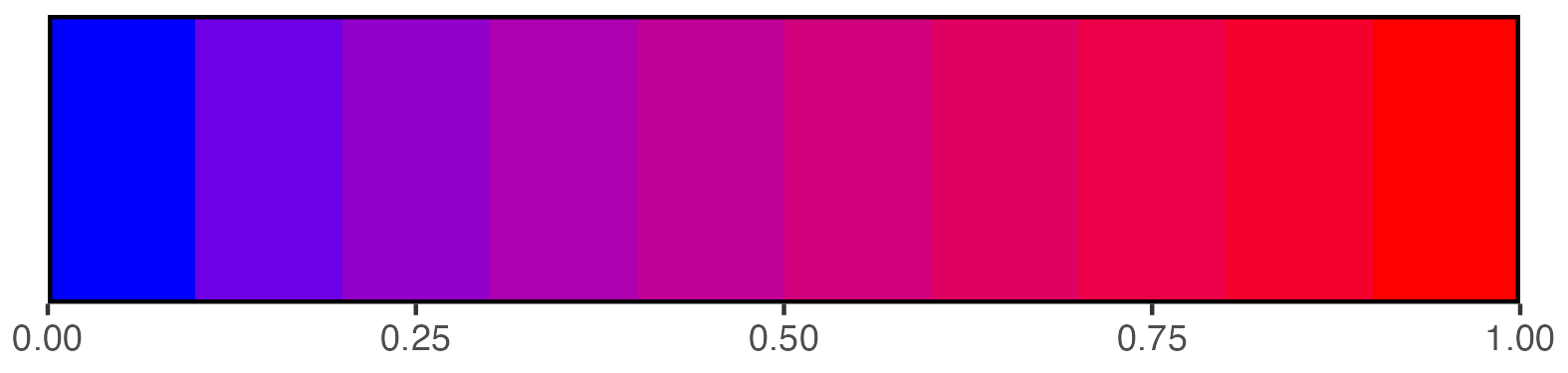
Disabling axis ticks with intermediate precision gives the following:
## Create scalebar and save to object
scalebar <- visualise_methylation_colour_scale(
    precision = 50,
    do_axis_ticks = FALSE
)

## Write png from object
ggsave(paste0(output_location, "modification_scalebar_alone_02.png"), scalebar, dpi = 300, width = 5.25, height = 1.25, device = ragg::agg_png)

## View image
view_image(paste0(display_location, "modification_scalebar_alone_02.png"))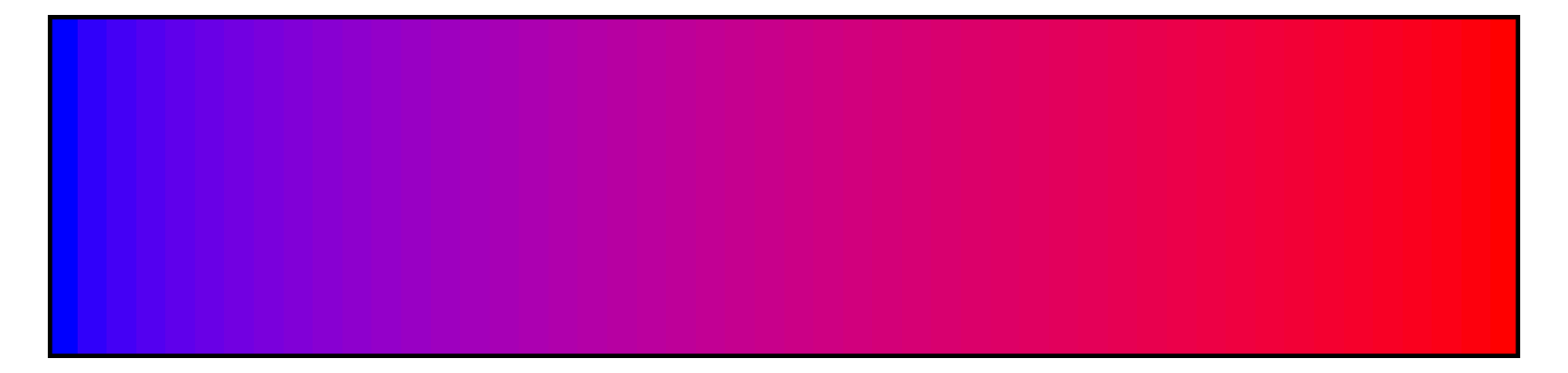
If ticks are left on, they can be customised with scale_x_continuous() as per usual for a ggplot. Here is an example of the left side being the gradient axis i.e. a vertical plot, with ticks every 0.1 instead of every 0.25.
## Create scalebar and save to object
scalebar <- visualise_methylation_colour_scale(
    high_colour = "green",
    low_colour = "yellow",
    high_clamp = 0.8,
    low_clamp = 0.5,
    full_range = c(0,1),
    precision = 101,
    axis_location = "left",
    do_axis_ticks = TRUE,
    axis_title = "some kind of title",
    outline_colour = "red",
    outline_linewidth = 3
) +
    scale_x_continuous(breaks = seq(0, 1, 0.1))

## Write png from object
ggsave(paste0(output_location, "modification_scalebar_alone_03.png"), scalebar, dpi = 300, width = 2, height = 5.25, device = ragg::agg_png)

## View image
view_image(paste0(display_location, "modification_scalebar_alone_03.png"))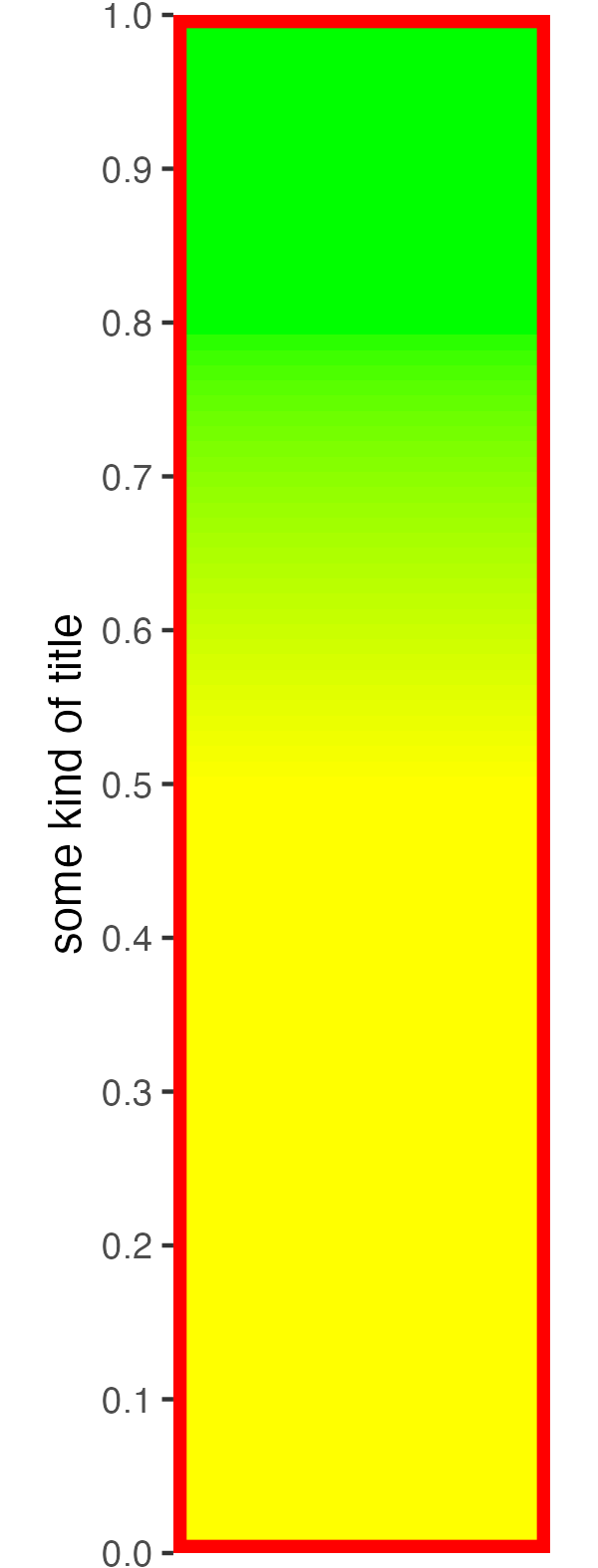
And here is an example of a more sensible scalebar with top text:
## Create scalebar and save to object
scalebar <- visualise_methylation_colour_scale(
    low_clamp = 0.1*255,
    high_clamp  = 0.9*255,
    axis_location = "north",
    axis_title = "Methylation probability",
    outline_linewidth = 0
)

## Write png from object
ggsave(paste0(output_location, "modification_scalebar_alone_04.png"), scalebar, dpi = 300, width = 5.25, height = 2, device = ragg::agg_png)

## View image
view_image(paste0(display_location, "modification_scalebar_alone_04.png"))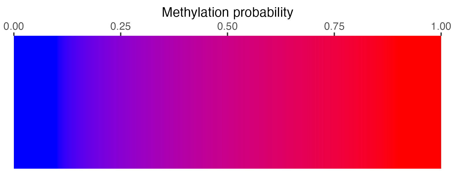
6.8 Think about the offset!
When merging modification data read from FASTQ, the positional offset when reversing can be changed (as discussed in detail in the reading from modified FASTQ section).
A summary of the sensible offset options (i.e. 0 or 1) copied from that section is as follows:
## Here the stars represent the true biochemical modifications on the reverse strand:
## (occurring at the Cs of CGs in the 5'-3' direction)
##
##
## 5'  GGCGGCGGCGGCGGCGGA  3'
## 3'  CCGCCGCCGCCGCCGCCT  5'
##        *  *  *  *  *

## If we take the complementary locations on the forward strand,
## the modification locations correspond to Gs rather than Cs,
## but are in the exact same locations:
##
##        o  o  o  o  o
## 5'  GGCGGCGGCGGCGGCGGA  3'
## 3'  CCGCCGCCGCCGCCGCCT  5'
##        *  *  *  *  *

## If we offset the locations by 1 on the forward strand,
## the modifications are always associated with the C of a CG,
## but the locations are moved slightly:
##
##       o  o  o  o  o
## 5'  GGCGGCGGCGGCGGCGGA  3'
## 3'  CCGCCGCCGCCGCCGCCT  5'
##        *  *  *  *  *
The visualisations thus far in this section have all used offset = 1 so that methylated Cs in CGs on the reverse strand are mapped to Cs of CGs in the forward strand when reverse complemented, ensuring consistency with reads that were forward to begin with.
However, there are actually four ways reverse read may be displayed: - All reads 5’-3’, with reverse reads running the opposite direction to forward reads (accomplished by not using the forward_<sequence/locations/probabilities> columns in extract_and_sort_methylation(), so that the raw unreversed reads are shown). - Reverse reads flipped to 3’-5’ so that they are complementary to the forward reads (accomplished by setting reverse_complement_mode = "reverse_only" and offset = 0 in merge_methylation_with_metadata()) - Reverse reads reverse-complemented to the corresponding 5’-3’ so that they match the forward reads, but leaving modifications in the original locations i.e. G of the reversed CG dinucleotides (accomplished by setting reverse_complement_mode = "DNA" and offset = 0 in merge_methylation_with_metadata()). - Reverse reads reverse-complemented to the corresponding 5’-3’ so that they match the forward reads, and offsetting the modification locations by 1 to always be on the C of CG dinucleotides even after reverse-complementing (accomplished by setting reverse_complement_mode = "DNA" and offset = 1 in merge_methylation_with_metadata()).
To illustrate this, we will create a dataset of two reads over the same region but in opposite directions, and apply each of these four extraction options. This will also serve to illustrate how ggDNAvis visualisations can be returned as ggplot objects and further modified:
## Create random methylation probabilities
set.seed(1234)
random_probabilities <- sample(0:255, size = 12, replace = TRUE)

## Set up original dataframe with reads always 5'-3'
location_reversing_example <- data.frame(
    read = c("example_f", "example_r"),
    sequence = c("GGCGGCGGCGGCGGAGGAGGCGGCGGAGGAA", "TTCCTCCGCCGCCTCCTCCGCCGCCGCCGCC"),
    quality  = rep("BBBBBBBBBBBBBBBBBBBBBBBBBBBBBBB", 2),
    sequence_length = rep(31, 2),
    modification_types = rep("methylation", 2),
    methylation_locations = c("3,6,9,12,21,24", "7,10,19,22,25,28"),
    methylation_probabilities = c(vector_to_string(random_probabilities[1:6]), vector_to_string(random_probabilities[7:12]))
)

## Set up metadata
location_reversing_metadata <- data.frame(
    read = c("example_f", "example_r"),
    direction = c("forward", "reverse")
)

## Create new dataframes with various reversal settings and save all to list
## Use c(list(original_dataframe), new_list) to make list of original then the three new ones
offsets <- c(0, 0, 1)
modes <- c("reverse_only", "DNA", "DNA")
dataframes <- c(list(location_reversing_example), lapply(seq_along(offsets), function(i) {
    reversed_data <- merge_methylation_with_metadata(
        location_reversing_example,
        location_reversing_metadata,
        reversed_location_offset = offsets[i],
        reverse_complement_mode = modes[i]
    )

    ## Overwrite "sequence" with "forward_sequence" etc in the returned dataframe
    ## This means "sequence" will hold the original sequences for the original dataframe,
    ## but hold the reversed/forwardified sequences for the following three dataframes
    reversed_data$sequence = reversed_data$forward_sequence
    reversed_data$methylation_locations = reversed_data$forward_methylation_locations
    reversed_data$methylation_probabilities = reversed_data$forward_methylation_probabilities

    return(reversed_data)
}))

## Extract locations/probabilities/sequences vectors from each dataframe
## Because of the overwriting at the previous step, "sequence", "modification_locations" etc
## hold the original values for the first (unmodified) dataset, but the forward-ified versions
## for the three later datasets
vectors_for_plotting <- lapply(dataframes, function(x) {
    extract_methylation_from_dataframe(
        x,
        locations_colname = "methylation_locations",
        probabilities_colname = "methylation_probabilities",
        sequences_colname = "sequence",
        lengths_colname = "sequence_length",
        grouping_levels = NA,
        sort_by = NA
    )
})

## Merge vectors across dataframes, with padding in between to visually separate the examples
blanks <- 3
input <- lapply(c("locations", "probabilities", "sequences"), function(x) {
    lapply(vectors_for_plotting, function(y) c(y[[x]], rep("", blanks))) %>%
        unlist() %>%
        head(-blanks) %>%
        c("", .)
})


## Calculate the tile width and height that we will end up with
lines_to_annotate <- 0:3*blanks + 1:4*2
margin = 0.5

k <- max(nchar(input[[3]]))
n <- length(input[[3]]) + length(lines_to_annotate)

## Create dataframe for titles
titles <- data.frame(
    text = c("(a) Original sequences, both 5'-3' (e.g. original reads):",
             "(b) Reversed to be 3'-5', offset 0:",
             "(c) Reverse-complemented to 5'-3' of other strand, offset 0:",
             "(d) Reverse-complemented to 5'-3' of other strand, offset 1:"),
    lines = lines_to_annotate - 1,
    x = 0
)
titles$y = 1 - (titles$lines - 0.66) / length(input[[1]])

## Create dataframe for 1 extra tile on each edge
## and for 5' and 3' direction indicators
lines_for_tiles <- sort(
    rep(seq_along(lines_to_annotate) + lines_to_annotate - 2, times = 2) +
    rep(0:1, each = length(lines_to_annotate)),
    decreasing = TRUE
)
directions <- data.frame(
    x = rep(c(-0.5, k+0.5) / k, each = length(lines_for_tiles)),
    y = rep((lines_for_tiles - 0.5 ) / n, times = 2),
    width = 1 / k,
    height = 1 / n,
    text = c(rep("5'", 2), "5'", "3'", rep("5'", 4),
             rep("3'", 2), "3'", "5'", rep("3'", 4))
)

## Create visualisation
output <- visualise_methylation(
    input[[1]],
    input[[2]],
    input[[3]],
    index_annotation_lines = lines_to_annotate,
    index_annotation_interval = 6,
    other_bases_outline_linewidth = 1,
    other_bases_outline_colour = "darkgrey",
    sequence_text_type = "sequence",
    index_annotation_always_first_base = FALSE,
    index_annotation_always_last_base = FALSE,
    low_clamp = 255*0.4,
    high_clamp = 255*0.6,
    margin = margin
) +
    ## Add titles and 5'/3' directions
    geom_tile(data = directions, aes(x = x, y = y, width = width, height = height), fill = alpha("white", 0), linewidth = 0) +
    geom_text(data = directions, aes(x = x, y = y, label = text), size = 15, col = "darkred", fontface = "bold") +
    geom_text(data = titles, aes(x = x, y = y, label = text), hjust = 0, size = 16)


## Save visualisation
ggsave(
    paste0(output_location, "modification_reversing_example.png"),
    plot = output,
    dpi = 100,
    ## k is the width in bases of the original visualisation
    ## We added 2 new squares, and need to account for the margin
    width = k + 2 + 2*margin,
    ## n is the height in bases of the original visualisation
    ## We didn't add any new lines, but still need to account for the margin
    height = n + 2*margin,
    device = ragg::agg_png
)

## View visualisation
view_image(paste0(display_location, "modification_reversing_example.png"))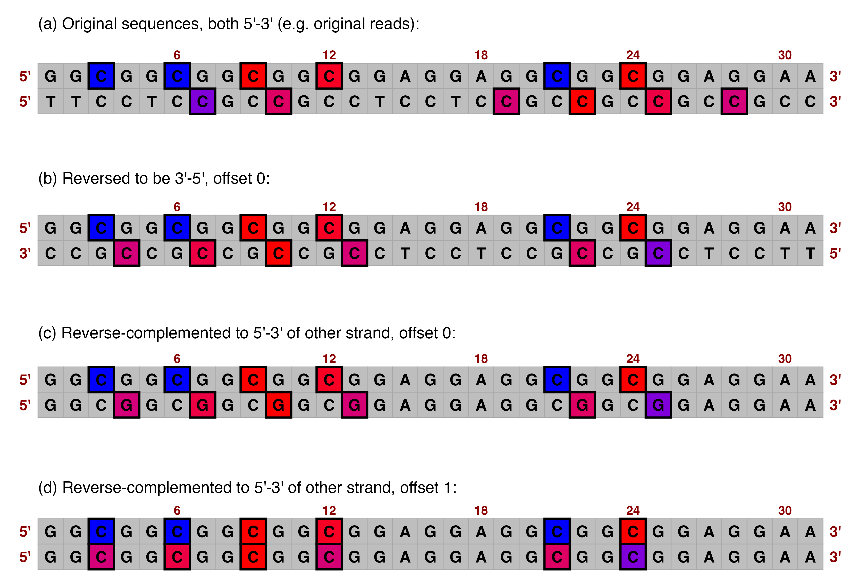
6.9 Performance
visualise_methylation() is identical to visualise_many_sequences() with respect to geom_raster() versus geom_tile(), so read visualise_many_sequences() performance.
For visualise_methylation(), geom_raster() is automatically used if:
-
sequence_text_typeis"none"orsequence_text_sizeis0, -
index_annotation_linesisNAornumeric(0), orindex_annotation_intervalis0, orindex_annotation_sizeis0, and - either:
-
outline_linewidthis0,modified_bases_outline_linewidthisNA, andother_bases_outline_linewidthisNA, or -
modified_bases_outline_linewidthis0andother_bases_outline_linewidthis0
-
7 Advanced usage
As ggDNAvis visualisations can be returned as ggplots by setting return = TRUE, they can be added to and further modified using standard ggplot processing (e.g. adding new geoms). The modification reversing example just above is one example of this, but more are shown in the ggDNAvis manuscript (Jade & Scotter, 2026) - not reproduced here for copyright safety. The code to generate all these advanced, composite visualisations is available in the manuscript/ directory of the source code repo.
The general principles of advanced usage are:
Visualisations can be returned using
return = TRUErather than being directly exported viafilename = "myfile.png".Additional layers such as text markup can be added in typical ggplot fashion, e.g. by making a new dataframe with text labels and locations (bearing in mind that ggDNAvis visualisations occupy a square from cartesian coordinates 0,0 to 1,1).
To export the images with the correct aspect ratio, you will need to calculate the appropriate dimensions. My approach is generally to count the width and height in bases (e.g.
width = max(nchar(sequences))andheight = length(sequences), though bear in mind that index annotations add additional lines e.g. might needheight = length(sequences) + length(index_annotation_lines)), then set those as the width and height in inches inggsave()while settingdpi = pixels_per_base.Composite/multi-panel visualisations can be made by merging ggplot objects using
patchworkorcowplotpackages, or by overlaying exported PNGs using themagickpackage.